Naturaleza en Hispania
http://naturalezaenhispania.com

“La existencia del mundo abre la mirada
del alma humana a la existencia de Dios.”
(Juan Pablo II, en Salvifici doloris)
Artículos
on-line de Documentos Aljibe
Edita: Sociedad
SURCOS, Avda. Torreón, nº 1 13001 Ciudad Real –
Depósito Legal: CR
820-1986- - ISBN 84-398-6347-0 ISSN 2445-1304 - Aviso Legal
Contacto:
Soledad López Fernández, solpfernandez@gmail.com
|
Volumen V |
Año:
2018 |
|
Artículo |
nº
8 |
|
Aceptado |
26
de junio 2018 |
Worldwide
Bioclimatology Manual and Guide
Manual
y Guía de Bioclimatología Mundial
Authors:
LOPEZ FERNANDEZ, MARIA LUISA – mllopez@unav.es (Departamento
de Biología Ambiental, Facultad de Ciencias, Universidad de Navarra), 31008
Pamplona.
LOPEZ, SOLEDAD – solpfernandez@gmail.com (Instituto de
Estudios Manchegos), 13002 Ciudad Real, España.
(English version, made by M.L. Lopez Fernandez,
of "Manual y Guía de
Bioclimatología Mundial, 2017", http://www.naturalezenhispania.com,
by the same authors).
ABSTRACT:
López, Fernández, M.L.& López
Fernández, M.S. (2018). “Worldwide
Bioclimatology Manual and Guide”. Documentos Aljibe “on-line”, vol. V, n.8., 26
de junio de 2018. Ciudad Real. Edita Sociedad Surcos. Depósito Legal: CR
820-1986- - ISBN 84-398-6347-0 ISSN 2445-1304. http://www.naturalezenhispania.com.
A summary exposition of Rivas-Martínez & al. (2011)
“Worldwide Bioclimatic Classification System, Global Bioclimatics", is
given. We comment, usually in their own words, on the originality of its premises, its basic elements, its hierarchical levels, its Isobioclimates, the Ombroclimographes
(or Ombrolimogrames), and the Synoptic
Table of the Bioclimatic Classification of the Earth. With the help of the
information contained in the web: “http://www.globalbioclimatics.org”, Rivas-Mart. & Rivas-Sáenz (1996-2017), an approach
to World Bioclimatic Diversity is given. Also, as a complement to the
theoretical exposition, a practical example of how to perform the Bioclimatic
Classification of a weather station is provided. Finally, the possibility of performing
bioclimatic thematic maps, is commented, with bibliographical mention of the
most recent maps. As for us, we have expanded the Bioclimatic Variants of
Rivas-Mart. et al. (2011), with the concept of Normal Variant. We have also
added some precisions to their concept of Steppic Variant. We give a glossary
of concepts, which, in the offered pdf file, indicates the pages in which each
of the terms is used.
Key words: Macrobioclimates, Bioclimates, Bioclimatic Variants, Bioclimatic Belts,
Thermotypes, Ombrotypes, Isobioclimates, Ombroclimograms, Continentality,
Steppicity, Submediterraneity, Global Bioclimatic Diversity, Bioclimatic Maps.
RESUMEN
López, Fernández, M.L.& López Fernández, M.S.
(2018). “Worldwide Bioclimatology Manual and Guide”. Documentos Aljibe “on-line”, vol. V, n.8., 26
de junio de 2018. Ciudad Real. Edita Sociedad Surcos. Depósito Legal: CR
820-1986- - ISBN 84-398-6347-0 ISSN 2445-1304. http://www.naturalezenhispania.com.
Se realiza una exposición resumida de la
Clasificación Bioclimática Mundial, "Global Bioclimatics", de
Rivas-Martínez & al. (2011), comentando, muchas veces con sus mismas
palabras, la originalidad de sus premisas,
sus elementos básicos, sus niveles jerárquicos, los Isobioclimas, los Ombroclimografos (u Ombroclimogramas), y la Tabla Sinóptica de la Clasificación Bioclimática de la Tierra. Con
ayuda de la información contenida en “http://www.globalbioclimatics.org”, Rivas-Mart.
& Rivas-Sáenz (1996-2017), se hace una aproximación a la Diversidad
Bioclimática Mundial. Así mismo se ofrece un ejemplo práctico de cómo realizar
la clasificación bioclimática de una estación meteorológica, que complementa la
exposición teórica. Para terminar, se comenta la posibilidad de realizar mapas
temáticos bioclimáticos, con mención bibliográfica de los más recientes. Por
nuestra parte, hemos ampliado las Variantes Bioclimáticas de Rivas-Mart. et al.
(2011), con el concepto de Variante Normal, así como también hemos añadido
algunas precisiones a su concepto de Variante Esteparia. El trabajo se acompaña
de un glosario de conceptos, que, en la versión PDF que se ofrece, indica la
página en que se utiliza cada uno de ellos.
Palabras clave: Macrobioclimas, Bioclimas, Variantes Bioclimáticas,
Pisos Bioclimáticos, Termotipos, Ombrotipos, Isobioclimas, Ombroclimograma,
Continentalidad, Estepicidad, Submediterraneidad, Diversidad Bioclimática
Mundial, Mapas Bioclimáticos.
General Index
1.- Introduction
2.- Premises of the classification
3.- Basic Elements for the Global Bioclimatic
Classification
4.- Worldwide Bioclimatic Classification
5.-
Bioclimatic Synopsis of the Earth
6.- Isobioclimates
7.- Bioclimograms
8.- Approach to Global Bioclimatic Diversity
9.- Assessment
of Summer Aridity, with examples
10.- ITC and Ci Calculations
11.- Practical example of
complete bioclimatic characterization of a meteorological station, and of the
use of the synoptic table
12.- Bioclimatic Cartography
13.- Paginated glossary
14.- Table of contents
15.- Bibliography
1.- INTRODUCTION
Bioclimatology
is the science that studies the relationship between climate and the
distribution of living beings and their communities on Earth.
Since
approximately 1987, Rivas-Martínez has developed a new "Bioclimatic
Classification of the Earth", the "GLOBAL BIOCLIMATICS" of
Rivas-Martínez (1987, 2004, 2008). Precisely, also in 2008, López Fernández
& López Fernández published a "Guide to Recognizing and Classifying
Bioclimatic Units", with the aim of facilitating the understanding and use
of Rivas-Martínez's "Global Bioclimatics".
Recently,
Rivas-Martínez & al., 2011, have remodeled and completed the "Global
Bioclimatics", also called "Worldwide Bioclimatic Classification
System", which exclusively uses climatic data. The Worldwide Bioclimatic
Classification, by Rivas Martínez & al., is hierarchical and recognizes
three levels: Macrobioclimate, Bioclimate / Variant, and Bioclimatic Belt -
consisting of a Thermotype and a Ombrotype.This new Bioclimatic Classification
recognizes in the Earth 5 Macrobioclimates, to which are subordinated 28
Bioclimates - in each one of which operate one or more of the nine recognized
Bioclimatic Variants, and, in addition, 31 Thermotypes and 9 Ombrotypes:
Altogether, over 400 elemental bioclimatic combinations, known as
Isobioclimates, each of one consisting of a Macrobioclimate, a Bioclimate /
Variant and a Bioclimatic Belt (a Thermotype plus an Ombrotype), which have
territorial representation in the Geobiosphere.
With this
"Manual and Guide to World Bioclimatology", we aim to facilitate the
understanding and use of this bioclimatic classification tool, so useful to
explain and understand Biogeography.
2.- PREMISES OF THE BIOCLIMATIC CLASSIFICATION OF THE
EARTH, RIVAS-MARTÍNEZ & al. (2011)
The following
eight premises bring together the main lines of force that condition the
distribution of life, as interpreted by Rivas-Martínez (2008) and
Rivas-Martínez & al. (2011), so they are at the basis of their Earth's
Bioclimatic Classification.
2.1. Reciprocity: In Bioclimatology, it has been shown that there is
an adjusted and reciprocal relationship between climate, vegetation and
geographical territories, ie, between Isobioclimates, biocenosis and
biogeographical units. This is because the distribution of vegetation, as well
as the evolution of the biocenosis, have accompanied and accompany the climatic
oscillations and the geological variations of the earth, which have taken place
in the past. (Exceptionally, some high alpine ridges have prevented vegetation
migrations and that reciprocity: see premise 8: Orogenies, below)
2.2. Photoperiod / Latitude: In the distribution of life have great influence,
both the photoperiod and its variation throughout the year, as well as the
angle with which the sun's rays affect the surface of the Earth, both phenomena
controlled by latitude. Therefore, latitude is the first factor used to
characterize and differentiate Macrobioclimates.
2.3. Continentality / Oceanicity - Annual thermal amplitude: The annual thermal
amplitude has an influence of first magnitude in the distribution of the
biocenosis and, consequently, in the borders of many Bioclimates. In the
Synoptic Table of the Earth's Bioclimatic Classification (see Figure 7, below),
it can be seen how the Continentality is used to differentiate the Temperate
Macrobioclimate from the Boreal Macrobioclimate, as well as all the Bioclimates
from each other except the Tropical.
2.4. Seasonality of Precipitation: The annual rhythm of precipitation has as much or
more importance, in the composition and distribution of the biocenosis, than
the amount of rain itself. The annual rhythm is the distribution of
precipitation throughout the year. Seasonality differentiates bioclimatic units
of several ranges: Macrobioclimates, Bioclimates and Bioclimatic Variants.
2.5. Mediterraneity: There is a large Mediterranean Macrobioclimate,
latitudinally extratropical, ombrically antithetical to the Tropical, Temperate
and Boreal Macrobioclimates, showing a summer aridity (or summer drought) of at
least two consecutive months: That is to say, in which the sum of the
precipitations of the two consecutive driest months of the summer quarter is
less than or equal to twice the sum of the average monthly temperatures of
those same months: (Psi + Psii) ![]() 2 ( Tsi + Tsii), being si
and sii the two consecutive months
drier of the summer. Such a shortage of rain during the summer, which can last
up to the twelve months of the year, is a brake for life, just during the
months thermally more favorable to growth. This circumstance is reflected in
deep physiognomic changes of the biocenosis, with respect to other Bioclimates
with precipitations of similar quantity, but without summer drought.
2 ( Tsi + Tsii), being si
and sii the two consecutive months
drier of the summer. Such a shortage of rain during the summer, which can last
up to the twelve months of the year, is a brake for life, just during the
months thermally more favorable to growth. This circumstance is reflected in
deep physiognomic changes of the biocenosis, with respect to other Bioclimates
with precipitations of similar quantity, but without summer drought.
2.6. Deserts: The deserts are the response of life to extremely
unfavorable climatic conditions, either by cold, or by aridity, or by both.
That is why there is no single type of desert bioclimate for all the deserts of
the world, but there are cold deserts, in all Macrobioclimates, and warm
deserts, in the Tropical and Mediterranean Macrobioclimates. In warm deserts,
the rate of precipitation is decisive, with maximums in summer - tropical
deserts - or in autumn and spring – Mediterranean deserts. The flora and
vegetation of both types of deserts are clearly different and are phenologically
adapted to the precipitation rhythms.
2.7. Oroclimates (Mountain climates): In the mountains, the Bioclimate, except for
temperature and precipitation values, shows a close relationship, in the
photoperiod values, with that of its piedmont. Therefore, in the mountains,
just as there is a certain vertical zonation of the biocenosis, there is also,
for each Macrobioclimate, a particular sequence of thermotypic and ombrotypic
combinations, that is to say, a particular sequence of Bioclimatic Belts. So
that the altitudinal succession of vegetation floors is explained by thermal
and ombric changes due to altitudinal and / or exposure-orientation changes.
2.8. Orogenies: In some regions of the Earth, paleogeological,
orographic and paleoclimatic circumstances have prevented the free migration of
the biocenosis, in correspondence with the climatic variations that were
occurring. Therefore, in those regions, the reciprocal relationship between
climate and distribution of the biocenosis, announced in the first Premise, can
not be met. One such circumstance has been the Alpine orogeny, which gave rise
to an almost continuous set of high mountain systems oriented East-West (Hindu
Kush, Himalayan, Tibet and Karakorum, etc.) on the Asian continent. These reliefs,
of considerable altitude, have acted as a barrier, greatly limiting the
migratory movements of life forms, during the great climatic changes that
followed. Thus, in addition to the severe extinctions during arid or glacial
periods, these large Central Asian transverse ridges have prevented the
biocenotic recolonizations from the adjacent subtropical belt during the
interglacial and, ultimately, during the Holocene periods. As a consequence,
between the meridians 70º and 110º E, and between the 25º and 35º N parallels,
it was necessary to establish the altitudinal limit of 2,000 meters, as an
approximate border between the Tropical Macrobioclimate on the one hand, and
the Mediterranean and Temperate Macrobioclimates, on the other.
3.- BASIC COMPONENTS FOR THE WORLDWIDE BIOCLIMATIC
CLASSIFICATION
After having
seen the Premises that underpin this Worldwide Bioclimatology, we will now
comment on its basic elements, namely: Latitude, Annual distribution of
rainfall, Bioclimatic Parameters, and Bioclimatic Indices.
All the
necessary data for the Bioclimatic Classification of the Earth are offered even
by the simplest thermopluviometric stations. These are the following data: Name
and Country; Latitude, Longitude and Altitude; period of temperature and precipitation
observations; monthly averages of maximum and minimum temperatures; and monthly
rainfall. In total, 43 data are needed from each meteorological station.
However, let us
note that the great work of Rivas-Martínez and his team has been the double selection
they have achieved: First, they have selected the parameters and indices that
are significant for the distribution of life and which are easily obtained from
the 43 basic data provided by the meteorological stations; And secondly, they
have once again made a successful selection by assigning, at each step of the
bioclimatic hierarchical classification, those parameters and indices that make
it possible to differentiate these levels. All these selections are not
subjective, but have been made by relating the different types of ecosystems to
the climatological data offered by the stations (more than 20,000, worldwide,
collected by Rivas Martínez, in the database of his Phytosociological Research
Center, Spain, http://globalbioclimatics.org/).
In doing so, the
predictive value of the result, that is, of the World Bioclimatic
Classification, is truly astounding. But in reality, what should astound us is
the knowledge of the different forms of life and their distribution-geographic
positioning at world-wide level, and the work of relating that knowledge with
the climatic data.
Next, we will
discuss the following five topics:
3.1.- Latitude: Latitudinal
Zones and Bands.
3.2.- Seasonality of
temperatures and rainfall. Period of plant activity. Types of frost.
3.3.- Parameters
3.3.1.- Seasonal Parameters
3.3.2.- Temperature
Parameters
3.3.3.- Precipitation
Parameters
3.4.- Bioclimatic Indexes
3.4.1.- Continentality /
Oceanicity Index: Annual thermal amplitude - lc -
3.4.2.- Index of Thermicity It and Index of Compensated Thermicity Itc
3.4.3.- Ombrothermal Indexes
- Io -
3.5.- Alphabetical list of
the abbreviations that designate the Parameters and the Bioclimatic Indexes.
3.1.- Latitude: Latitudinal Zones and Waists.
The three
factors that most influence the distribution of life - the photoperiod and its
annual variation, the temperature and its seasonal variation, and the amount of
precipitation along with its annual rhythm - have a close correlation with the
values of latitude. It is therefore not surprising that the limits of the
superior bioclimatic units in World Bioclimatology show a close correspondence
with the latitudinal zones and bands traditionally proposed by geographers. In
figure 1 we show the latitudinal Zones and Bands, for later, in figure 3, to
point out and comment their correlations with the Macrobioclimates.
Latitudinal Zones. -In terms of latitude, at any altitude above sea
level, large latitudinal zones are distinguished on Earth (see Rivas-Mart et
al., 2011): one Warm – between the 35º North and South; two Temperate - between
the 35º-66º N and S; and two Cold- between 66º-90º N and S.
Figure 1. Amplitude of latitudinal Zones and Belts
recognized on Earth (according to Rivas-Mart et al., 2011):
|
|
Latitudinal
Zones |
Latitudinal Belts |
|
|
N |
3. Cold 66º-90º |
3a. Arctic
66º-90º |
|
|
2. Temperate 35º-66º |
2b. Subtemperate 51º-66º |
||
|
2a. Eutemperate 35º-51º |
|||
|
1. Warm 0º-35º |
1c. Subtropical 23º-35º |
||
|
1b. Eutropical 7º-23º |
|||
|
1a. Equatorial 7ºN-7ºS |
|||
|
S |
1. Warm 0º-35º |
||
|
1b. Eutropical 7º-23º |
|||
|
1c. Subtropical 23º-35º |
|||
|
2. Temperate 35º-66 |
2a. Eutemperate 35º-51º |
||
|
2b. Subtemperate 51º-66º |
|||
|
3. Cold 66º-90º |
3a. Antartic 66º-90º |
Latitudinal Belts. - Depending on the latitude, at any altitude above
sea level, 11 wide latitudinal belts are distinguished on Earth:
In the Warm
Zone, the following 5 latitudinal Belts are recognized: one Equatorial
Belt, 7º North - 7º South; two Eutropical Belts, 7º-23º North and 7º- 23º
South; and two Subtropical Belts, 23º-35º North and 23º-35º South.
In the Temperate
Zones, which contact north and south with the warm zone, 4 latitudinal
belts are recognized: two Eutemperate Belts, 35º-51º North and 35º-51º South;
and two Subtemperate Belts, 51º-66º North and 51º-66º South.
In the Cold
Zones, which contact both in the North and the South with the Temperate
zones, only two latitudinal belts are recognized, one Arctic belt, 66º-90º
North and another Antarctic belt, 66º-90º South.
3.2.- Seasonality of temperatures and rainfall. Period
of plant activity. Types of frost.
Seasonality
refers to variations in temperature and precipitation occurring throughout the
year. In tropical climates, seasonality is marked by precipitation, while, in
the extratropical climates, seasonality is marked by temperatures.
The seasonality
of temperatures and of precipitations is involved in the definition and
formulation of most of the Parameters and Indexes used in this Worldwide
Bioclimatic Classification, as we will see below. In fact, the seasonality of
temperatures and the amount of monthly precipitation, as well as its annual
rhythm, are data of great diagnostic value in the recognition and delimitation
of Macrobioclimates, Bioclimates
One aspect of
the seasonality of temperatures is the concept of "Plant activity
period". "Plant activity period" is the number of months whose
average monthly temperature exceeds a certain threshold to allow the
biochemical activity of plants. The most accepted threshold is Ti> 3ºC. Another aspect of the
seasonality of temperatures is the concept of "Types of frost", which
may be: absent, probable or sure, depending on the magnitude of the parameters mi and m'i. It is said that a month has frost absent, when its m'i> 0; it is said that a month has
probable frost, when it simultaneously fulfills mi> 0, and m'i ≤ 0;
and finally, it is said that one month has sure frost, if mi ≤ 0.
3.3.- Parameters
We understand by
Parameters the data or significant values of those climatic variables that are
considered necessary to analyze a bioclimatic situation.
In order to
establish this Worldwide Bioclimatic Classification, climatic data that are
easily accessible have been used - average monthly temperatures of the maximum
and minimum, and average monthly temperatures, expressed in degrees centigrade
(ºC), and monthly precipitations expressed in millimeters (mm). All these data,
which we consider as Parameters in this classification, are offered even by the
simplest weather stations, which, altogether, form a wide network around the
world.
The main
Parameters of seasonality, temperature and precipitation used in this
"Bioclimatic Classification of the Earth" are listed below by their
acronyms and notations. (For more information, see Rivas-Mart et al., 2011):
3.3.- Parameters
3.3.1. – Seasonal Parameters
3.3.2.- Temperature
Parameters
3.3.3.- Precipitation
Parameters
3.3.1.- Seasonal Parameters
The sequence of
atmospheric changes, and their duration, are of paramount importance to life.
Therefore, in Bioclimatology, it is interesting to take into account the
following periods of time - Seasonal parameters - during which vegetation and
flora are especially sensitive to certain climatic values of temperature and
precipitation.
We list the main
Seasonal Parameters used in this Classification. From each one its acronym and
its contents are indicated:
Tr1 Winter solstice trimester. Season: Winter (W, Winter).
Dec-Jan-Feb, latitude N; Jun-Jul-Aug, latitude S.
Tr2 Spring equinox trimester. Season: Spring (P, Spring).
Mar-Abr-May, latitude N; Sep-Oct-Nov, latitude S.
Tr3 Summer solstice trimester. Season: Summer (S, Summer).
Jun-Jul-Aug, latitude N; Dec-Jan-Feb, latitude S.
Tr4 Autumn equinox trimester. Season: Autumn (F, Fall, Automn).
Sep-Oct-Nov, latitude N; Mar-Abr-May, latitude S.
Cm1 The warmest four-month period of the year.
Cm2 Four-month period following the Cm1.
Cm3 Four-month period prior to the Cm1.
Pav Period of plant physiological activity: number of months whose
average monthly temperature equals or exceeds 3.5ºC: Ti ≥ 3,5ºC.
Pf Periods of frost: number of months with frost absent,
probable or safe.
Ss Warmer semester of the year
Sw Warmer semester of the year
3.3.2.- Temperature
Parameters
Are data, annual
or monthly, of temperatura. We list them by their initials, indicating their
content. Average temperatures are expressed in degrees centigrade and positive
temperatures, in tenths of a degree centigrade.
T Average annual temperature
Ti Average monthly temperature, standing:
1 = January, ..., 12 = December
Tmax Average monthly temperature of the warmest month of the year
Tmin Average monthly temperature of the coldest month of the year.
Tp Positive Annual Temperature: Quantifies, for each place, the
thermal energy available for life. It is the sum, expressed in tenths of degree
centigrade, of the average monthly temperatures of those months that exceed
0ºC: Tp= ![]()
Tps Positive Temperature of the warmest trimester of the year
(Tropical Macrobioclimate), or summer trimester (Macrobioclimates
extratropical), expressed in tenths of degree centigrade.
Tpw Positive Temperature of the coldest trimester of the year,
expressed in tenths of degree centigrade.
Tsi Monthly Medium Temperature of any Summer
month
M Average temperature of the maximum temperatures of the
coldest month in the year, ie, the month with the lowest Ti.
m Average temperature of the minimum temperatures of the
coldest month in the year, that is, the month with the lowest Ti.
mi Average monthly temperature of the mínimum temperatures,
where i: 1 = January, ..., 12 = December.
m’i Average monthly temperature of absolute minimum temperatures,
where i: 1 = January, ..., 12 = December.
3.3.3.- Precipitation Parameters.
They are
expressed in mm (or liters per square meter):
P Annual precipitation.
Pi Monthly precipitation, where i: 1 = January, ..., 12 =
December.
Pss Precipitation of the six warmest months of the year
Psw Precipitation of the coldest six months of the year
Pcm1 Precipitation of the warmest four-month period of the year.
Pcm2 Precipitation of the four months period following the warmest
four-month period of the year.
Pcm3 Precipitation
of the four months period previous to the warmest four months period of the
year.
P Tr1 Precipitation of the winter solstice trimester. Season: Winter (W,
Winter). Dec-Jan-Feb, latitude N; Jun-Jul-Ago, latitude S.
P Tr2 Precipitation of the spring equinox trimester. Season: Spring (P,
Spring). Mar-Abr-May, latitude N; Sep-Oct-Nov, latitude S.
P Tr3 Precipitation of the summer solstice trimester. Season: Summer (S,
Summer). Jun-Jul-Aug, latitude N; Dec-Jan-Feb, latitude S.
P Tr4 Precipitation of the automn equinox trimester. Season: Autumn (F,
Fall, Automn). Sep-Oct-Nov, latitude N; Mar-Abr-May, latitude S.
Ps Precipitation of the summer trimester -S, Summer.
Jun-Jul-Aug, latitude N; Dec-Jan-Feb, latitude S.
Psi Monthly precipitation of any Summer month
Pw Winter trimester precipitation -W, Winter. Dec-Jan-Feb,
latitude N; Jun-Jul-Ago, latitude S.
Psb1 Precipitation of the first two months after the summer solstice
(July-August in latitude N, January-February in latitude S)
Psb2 Precipitation of the two subsequent months to Psb1
(September-October in latitude N, March-April in latitude S)
Pp Annual Positive Precipitation: Pp = ∑Pi (Ti>0ºC). Pp is the sum of Pi of all months of the year, whose Ti is greater than 0ºC. Pp=∑Pi (Ti>0), being i: 1 = January, ..., 12 = December.
Pps Positive Precipitation of the three warmest months period of
the year (tropical zones), or of the summer trimester (extratropical zones).
Ppw Positive Precipitation of the three coldest months period of the
year (tropical zones), or of the winter trimester (extratropical zones).
> W> Winter precipitation.
> P> Spring precipitation.
> S> Summer precipitation.
> F> Fall precipitation.
3.4.- Bioclimatic Indexes
3.4.1.- Continentality
/ Oceanicity Index: Annual thermal amplitude -lc-
3.4.2.- Thermicity
Index -It- and Compensated Thermicity Index -Itc-
3.4.3.- Ombrothermic
Indexes -Io-
The indexes are
the result of applying simple arithmetic formulas to various parameters of
rainfall and / or temperature, selected by seasonal criteria or by criteria of
specific biological requirements.
For
this classification, Rivas-Martínez (2008) and Rivas-Martínez et al. (2011)
have selected some Indexes, such as Continentality Index, already proposed by
other authors, but, above all, they have created other new Indexes -the
Thermicity Index as well as the Ombrothermic Indexes- which have great
prediction capacity with respect to the distribution of the life.
It
is precisely in the discovery of new Bioclimatic Indexes that the most
brilliant part of the bioclimatic system of Rivas-Martínez (2008) and
Rivas-Martínez et al. (2011), as we have already said. To discover and
establish them, interpreting and following the dictation of the distribution of
life and its dynamism, they have used all the ideas and demands contained in
the Premises and the Basic Elements, already commented. They have also handled
climate data from 20,000 stations around the world, which obviously reduces the
subjectivism of choice.
3.4.1.- Continentality / Oceanicity Index: Annual
thermal amplitude -lc-
The
Continentality / Oceanity Index quantifies the amplitude of the annual thermal
oscillation by calculating the thermal interval between the highest and lowest
monthly average temperatures of the year. Although the index is called
"Continentality Index", if its values are between 0 and 21,
traditionally we talk about Oceanity, while, if they are high, over 21, we talk
about Continentality. This Continentality Index, despite its simplicity, shows
an excellent correlation with life. In addition, the data required for its
calculation are provided by all weather stations, even the simplest ones.
The
Continentality / Oceanity index expresses the difference, in degrees
centigrade, between the highest and lowest monthly average temperatures of the
year:
Ic
= Tmax – Tmin
The Continentality Types and Subtypes recognized in
the "Bioclimatic Classification of the Earth, together with their Ic
intervals, are shown in Figure 1A.
Figura
1A. Types and Subtypes of Continentality, and their intervals of Ic.
|
TYPES |
Ic VALUES |
SUBTYPES |
Ic VALUES |
|
Hyperoceanic |
0≤Ic≤11 |
1.1 Ultrahyperoceanic |
0≤Ic≤4 |
|
1.2 Euhyperoceanic |
4<Ic≤8 |
||
|
1.3 Subhyperoceanic |
8<Ic≤11 |
||
|
Oceanic |
11<Ic≤21 |
2.1 Semihyperoceanic |
11<Ic≤14 |
|
2.1 Euoceanic |
14<Ic≤17 |
||
|
2.3 Semicontinental |
17<Ic≤21 |
||
|
Continental |
21<Ic≤66 |
3.1 Subcontinental |
21<Ic≤28 |
|
3.2 Eucontinental |
28<Ic≤46 |
||
|
3.3 Hypercontinental |
46<Ic≤66 |
3.4.2.- Index of Thermicity -It- and Index of
Thermicity Compensated -Itc-
The Thermicity Index weighs and quantifies
the intensity of the winter cold, a limiting factor for many types of life. It
is calculated by summing T (mean annual temperature), M (mean temperature of
the maximum of the coldest month), and m (mean temperature of the minimum of
the coldest month), and expressed in tenths of a degree centigrade:
It = (T + M + m) 10
It is,
therefore, an Index that considers together the intensity of the winter cold
and the average annual temperature.
But since (M
+ m) is approximately, ≈2Tmin (Tmin = average temperature of the coldest month of the year), it is
not necessary to know neither M nor m, to calculate It:
It
≈ (T + 2 Tmin) 10
The correlation of this Thermicity Index with
vegetation is very satisfactory in countries with warm and temperate climates.
However, in cold countries, or in countries with a continental tendency, the
relationship with vegetation is more precise if the Annual Positive Temperature
(Tp) is used. For this reason, it is
a very useful Index to distinguish the Tropical Macrobioclimate from the Mediterranean
and Temperate Macrobioclimetes, in those latitudes in which the three
Macrobioclimates coincide (latitudes above 23 N and S). In the Mediterranean
and Temperate Macrobioclimates, unlike in the Tropical, there is the winter:
therefore, their lt is necessarily
lower than in the Tropical.
Compensated Termicity Index.
As the
Thermicity Index is greatly affected by the annual thermal amplitude -
Continental Index, lc-, it needs a certain compensation, to make possible the
comparisons between localities, regardless of the excesses of temperance or
cold, that occur in hyperoceanic climates, or in the hypercontinental ones. It
has been thus arrived at the Compensated Thermicity Index - Itc - which is no more than the value
of It plus a compensation value, Ci:
Itc
= It + Ci
Value
of Ci.
Ci is the compensation value
to correct for the excess "temperance" or "cold" occurring
in extratropical areas (more than 23 ° N and S), when the Continental Index is
extremely low (Ic ≤ 8), or high (Ic> 17), compared to cases where Ic
has mean values: In this way, the effect
of an "excess" Ocean / Continental, on the measure of the climate
thermal comfort, is neutralized. The value of Ci is calculated according to latitude and Continentality. Chapter
10 details the procedure for calculating Itc
and Ci, with the help of several
examples of stations with different Continental Indexes. (See Chapter 10).
As the truly meaningful Index is the Compensated Thermicity Index, Itc, we will always speak, in this work,
of Itc. (In their study of the
world's weather stations, see www.globalbioclimatics.org (Rivas-Mart. &
Rivas-Sáenz, 1996-2017), authors indicate both It and Itc).
3.4.3.- Ombrothermic
Indexes -Io-
They serve to measure the moisture comfort that life
enjoys in the different terrestrial zones. The Ombrothermic Index relates the
precipitation to the temperature, but using the Parameters of Positive
Precipitation and Positive Temperature, already discussed. The value of an
Ombrothermic Index is the quotient between Positive Precipitation and Positive
Temperature of the considered period, multiplied by ten:
Io = (Pp/Tp) 10.
Certain
intervals of Io reflect faithfully changes in biocenosis. The Ombrothermic
Indexes are so determinant and significant that their intervals are used in all
hierarchical levels of the Bioclimatic Classification of the Earth of
Rivas-Martínez (2008) and Rivas-Martínez et al. (2011).
In addition to
the Io, Annual Ombrothermic Index,
many other Ombrothermic Indices can be calculated, for various periods that are
considered significant, of 1, 2, 3, or more months.
In tropical
territories, it is sometimes necessary to know the index:
Iod2 Ombrothermic
Index of the driest bimester within the driest four-month period of the year.
Among the various
Ombrothermic Indexes used in extratropical territories, the following are very
significant:
Ios, Iosi Ombrothermic
Index of any month of the summer trimester (Tr3)
Ios1 Ombrothermic Index of the hottest month of the summer
trimester (Tr3)
Ios2 Ombrothermic Index of the hottest bimester
of the summer trimester (Tr3)
Iosc Summer compensable Ombrothermic Indexes.
Two of them are considered:
Iosc3 (= Ios3): Compensable
Ombrothermic Index of the summer trimester (Tr3), necessary to evaluate the summer aridity
Iosc4 (= Ios4): Compensable Summer Ombrothermic Index for the
four-month period resulting from adding, to the summer trimester (Tr3), the month immediately preceding. This index is also
used to assess summer aridity.
All these Summer
Ombrothermic Indexes are very important, since they measure the summer aridity
and its possible compensation: They are essential to differentiate the
Mediterranean Macrobioclimate, from the Temperate and Boreal Macrobioclimates
(see these, sections 4.1.2, 4.1.3, and 4.1.4). For the correct use of all these
Indexes, see chapter 9.
3.5.- Alphabetical list of the abbreviations that
designate the Parameters and the Bioclimatic Indexes.
We have found it
necessary to list, in alphabetical order, all the Parameters and Indices
mentioned in the previous headings (See Figure 2).
Figure 2.
Alphabetical list of Parameters and Bioclimatic Indexes acronyms.
|
Para-meter /Index |
Descripción |
|
Ci |
Continentality
compensation value |
|
Cm1 |
The warmest four-month period of the year. |
|
Cm2 |
Four-month period following the Cm1 |
|
Cm3 |
Four-month period prior to the Cm1 |
|
Ic |
Continentality / Oceanicity Index: Annual thermal
amplitude. |
|
Io |
Annual Ombrothermal Index: (Pp/Tp) x 1O. |
|
Iod2 |
Ombrothermal Index of the driest bimester within the
driest four-month period of the year. |
|
Ios, Iosi |
Ombrothermal Index of any month of the summer
trimester |
|
Ios1 |
Ombrothermal Index of the hottest month of the
summer trimester (Tr3) |
|
Ios2 |
Ombrothermal Index of the hottest bimester of the
summer trimester (Tr3) |
|
Iosc |
Summer
compensable Ombrothermal Indexes |
|
Iosc3(= Ios3) |
Compensable Ombrothermic Index of the summer
trimester, necessary to evaluate the summer aridity |
|
Iosc4(= Ios4) |
Compensable Summer Ombrothermal Index for the
four-month period resulting from adding, to the summer trimester, the month
immediately preceding. This
index is also used to assess summer aridity. |
|
It |
Thermicity
Index |
|
Itc |
Compensated
Thermicity Index |
|
M |
Average temperature of the maximum temperatures of
the coldest month in the year, ie, the month with the lowest Ti. (Seasonal Temperature Index) |
|
m |
Average temperature of the minimum temperatures of
the coldest month in the year, that is, the month with the lowest Ti. (Seasonal Temperature Index) |
|
mi |
Average monthly temperature of the mínimum
temperatures, where i: 1 = January, ..., 12 = December. |
|
m´i |
Average monthly temperature of absolute minimum
temperatures, where i: 1 = January, ..., 12 = December |
|
P |
Annual
precipitation |
|
Pav |
Period of plant physiological activity |
|
Pcm1 |
Precipitation of the warmest four-month period of
the year. |
|
Pcm2 |
Precipitation of the four months period following
the warmest four-month period of the year |
|
Pcm3 |
Precipitation of the four months period previous to
the warmest four months period of the year |
|
Pf |
Periods
of frost |
|
Pi |
Monthly precipitation, where i: 1 = January, ..., 12
= December. (Weather
parameter) |
|
Pp |
Annual
Positive Precipitation |
|
Pps |
Positive Precipitation of the three warmest months period
of the year (tropical zones), or of the summer trimester (extratropical
zones). |
|
Ppw |
Positive Precipitation of the three coldest months
period of the year (tropical zones), or of the winter trimester
(extratropical zones). |
|
Ps |
Precipitation of the summer trimester |
|
Psb1 |
Precipitation of the first two months after the
summer solstice (July-August in latitude N, January-February in latitude S) |
|
Psb2 |
Precipitation of the two subsequent months to Psb1
(September-October in latitude N, March-April in latitude S) |
|
Psi |
Monthly precipitation of any Summer
month |
|
Pss |
Precipitation of the six warmest months of the year |
|
Psw |
Precipitation of the coldest six months of the year |
|
PTr1 |
Precipitation of the winter solstice trimester |
|
PTr2 |
Precipitation of the spring equinox trimester |
|
PTr3 |
Precipitation of the summer solstice trimester |
|
PTr4 |
Precipitation of the automn equinox trimester |
|
Pw |
Winter
trimester precipitation |
|
Ss |
Warmer semester of the year |
|
Sw |
Warmer semester of the year |
|
T |
Average annual temperature. (Weather parameter) |
|
Ti |
Average monthly temperature, standing: 1 = January,
..., 12 = December. (Weather
parameter) |
|
Tmax |
Average monthly temperature of the warmest month of
the year. |
|
Tmin |
Average monthly temperature of the coldest month of
the year. |
|
Tp |
Positive
Annual Temperature |
|
Tps |
Positive Temperature of the warmest trimester of the
year (Tropical Macrobioclimate), or summer trimester (Macrobioclimates
extratropical) |
|
Tpw |
Positive Temperature of the coldest trimester of the
year |
|
Tr1 |
Winter
solstice trimester |
|
Tr2 |
Spring
equinox trimester |
|
Tr3 |
Summer
solstice trimester |
|
Tr4 |
Autumn
equinox trimester |
|
Tsi |
Monthly Medium Temperature of any Summer
month |
|
>W> |
Winter
precipitation. |
|
>P> |
Spring
precipitation. |
|
>S> |
Summer
precipitation. |
|
>F> |
Fall
precipitation. |
4.- WORLDWIDE
BIOCLIMATIC CLASSIFICATION
The Worldwide
Bioclimatic Classification (Rivas-Mart, 2008, Rivas-Mart et al., 2011) is
necessarily hierarchical, because it has to reflect the different range of
influence of climatic factors on the distribution of life. The hierarchical
bioclimatic units of the Classification are: 1-Macrobioclimates, 2-Bioclimates
/ Variants, and 3-Bioclimatic Belts.
Latitude
has a decisive influence on the distribution of living beings and, for that
reason, it is used in the first hierarchical step of classification, that of
the Macrobioclimates. Indeed, latitude determines the photoperiod, the
inclination of the sun's rays, the distribution of high and low atmospheric
pressures, the general circulation of the atmosphere and its effect on the
amount and distribution of rainfall, etc.,
Likewise, in
each Macrobioclimate, the distribution patterns of the plant communities are
governed by combinations of Continentality levels, together with humidity
comfort levels: Ic and Io. Bioclimates and their variants are
thus defined.
And in each
Bioclimate / Variant unit, the combination of one level of ltc, -or of Tp -
(Thermotype) with another of Io
(Ombrotipo), reflects the actual distribution of vegetation types and, thus,
define the third hierarchical level of the classification, the Bioclimatic
Belts.
4.1.- First hierarchical
level of the Classification: Macrobioclimates
4.2.- Second hierarchical
level of the Classification: Bioclimates / Variants
4.3.-
Third hierarchical level of the Classification: Bioclimatic Belts -Thermotypes and
Ombrotypes-
4.1. First hierarchical level of the
Classificacion: Macrobioclimates
The
Macrobioclimates are the greater rank typological units of this Bioclimatic
Classification. These are synthetic biophysical models, delimited by certain
latitudinal and climatic values, that have a wide territorial jurisdiction and
that are related to the great types of climates, biomes, and biogeographic
regions, of the Earth. The five Macrobioclimates that are accepted in this
classification are: Tropical, Mediterranean, Temperate, Boreal and Polar.
To distinguish
the Macrobioclimates, the latitudinal values are the first to be taken into
account, and their limits are shown in figure 3: Tropical Macrobioclimate fits
the latitudinal warm zone (35 N & S); Mediterranean Macrobioclimate
participates in the warm and temperate zones (23º-52º N & S); Temperate
Macrobioclimate also participates in the warm zone and extends through almost
all the temperate zone (23º-66ºN and 23º-55º S); Boreal Macrobioclimate is
distributed throughout almost all the temperate zone and the cold zone, but has
an asymmetric latitudinal distribution (42º-72º N and 49º-56º S); finally, the
Polar Macrobioclimate is almost symmetrically distributed in the temperate zone
and throughout the cold zone (51º-90ºN and
53º-90ºS).
Figure
3. Width of latitudinal zones and belts recognized on Earth, and their
relationship to the distribution of Macrobioclimates. As can be seen, the
limits of the Macrobioclimates do not coincide exactly with the corresponding belts,
although they show close correspondences.
|
|
Latitudinal
Zones |
Latitudinal
Belts |
Macrobioclimates |
|||||
|
N |
3.
Cold 66º-90º |
3a. Arctic
66º-90º |
|
|
|
|
Polar 51º-90º |
|
|
Boreal 42º-72º |
||||||||
|
2.
Temperate 35º-66º |
2b.
Subtemperate 51º-66º |
Temperate 23º-66º |
||||||
|
2a.
Eutemperate 35º-51º |
Medite-rranean 23º-52º |
|||||||
|
|
||||||||
|
|
||||||||
|
1.
Warm 0º-35º |
1c.
Subtropical 23º-35º |
0º-35º Tropical 0-35º |
||||||
|
1b.
Eutropical 7º-23º |
|
|
||||||
|
1a.
Equatorial 7ºN-7ºS |
||||||||
|
S |
1.
Warm 0º-35º |
|||||||
|
1b.
Eutropical 7º-23º |
||||||||
|
1c.
Subtropical 23º-35º |
Medite-rranean 23º-52º |
Temperate 23º-55º |
||||||
|
2.
Temperate 35º-66 |
2a.
Eutemperate 35º-51º |
|
||||||
|
Boreal 49º-56º |
||||||||
|
2b.
Subtemperate 51º-66º |
|
|||||||
|
|
Polar 53º-90º |
|||||||
|
|
||||||||
|
3.
Cold 66º-90º |
3a. Antarctic
66º-90º |
|||||||
As shown in
Figure 3, and despite their denominations, the boundaries of the
Macrobioclimates do not correspond exactly to the Latitudinal Zones and Belts,
but the comparison with them helps to locate the areas of each Macrobioclimate
on the continents.
1.-In the latitudinal belts equatorial - 7ºN-7ºS - and eutropical -
7º-23ºN and S-, as the solar radiation is practically zenith and the duration
of the day and of the night vary little along the year, the Macrobioclimate, at
any altitude, regardless of temperature, is considered tropical.
2.- In the subtropical latitudinal belts - 23º-35º N and S -, depending
on the temperature and the rhythm of the precipitations throughout the year,
the territory is divided between the Tropical, Mediterranean and Temperate
Macrobioclimates.
3.-In the eu-temperate latitudinal belts -35º-52ºN and S-, the seasonal
photoperiods and the less energy received represent a severe border for plant
and animal life, which have to adapt to drought and cold of the Mediterranean,
Temperate or Boreal Macrobioclimates, depending on the rainfall rhythms and
thermal levels.
4.-In the latitudinal subtemperate belts -52º-66ºN and 52º-60ºS-, the
photoperiod and the thermicity establish new limits to the life, by the
necessary adaptations to the intense photoperiod and the intense cold, typical
of the Macrobioclimates Temperate, Boreal and Polar .
5.-In the latitudinal Arctic -66º-90ºN-and Antarctic -60º-90ºS- belts,
due to the great difference in the duration of day and night, and the little
thermal energy that is received during the solstices, life finds very severe
limitations. Therefore, at any latitude and altitude, the Macrobioclimate is
considered Polar.
In addition to
the latitude, in the differentiation of the Macrobioclimas several thermal
indices are used, in some cases related to the Continental Index, as well as
certain rainfall rhythms. Thus, the Compensated Thermicity Index, Itc, which
accurately measures the winter cold intensity - a true barrier for many living
beings - is very discriminant to differentiate tropical, Mediterranean and
temperate Macrobioclimates.
In the Earth's
Bioclimatic Synopsis, Figure 7, in the Macrobioclimates column, we find all the
necessary values to distinguish the Macrobioclimates from each other. Figure 4 is a copy of that first column of the
Earth's Bioclimatic Synopsis, which facilitates its consultation.
Note:
According to the Orobioclimates premise, to analyze the Macrobioclimate of a
meteostation located at a certain height above sea level, it is necessary to
theoretically calculate the thermal values that would have in its base, that
is, between 0 and 200 meters above sea level. For that, it is necessary to
increase T, M, Itc and Tp in certain values, for every 100 m that the weather
station exceeds 200m. The amount of the increments vary somewhat with the
latitude, so they are given, as a note, at the bottom of the summary table
"Bioclimatic Synopsis of the Earth". (See Figure 7)
Figure 4.- Column of Macrobioclimates,
extracted from the Bioclimatic Synopsis of the Earth
|
Macrobioclimates
(1) |
|
Name, Acronym and Differential Characters |
Tropical Tr
Warm Zone: Equatorial, Eutropical and Subtropical Belts (0º - 35º N
& S). In Subtropical (23º - 35º N & S) at < 200 m, at least two
values: T ≥ 25º, m ≥ 10º, Itc ≥ 580;
or, if Pss > Psw, or Pcm2 < Pcm1 > Pcm3,
at least two values: T ≥ 21º, M
≥ 18º, Itc ≥ 470. In Eurasia, from 25º to 35º N, height ≥ 2000 m: it is not tropical. |
Mediterranean
Me
Subtropical Warm Zone (23º to 35º N & S) and Eutemperate Temperate
Zone (35º to 52º N & S), with summer aridity at least bimonthly after the
summer solstice: Ios2 ≤ 2,
Iosc4 ≤ 2. In
the Subtropical, at least two of the three thermal values: T < 25º, m <
10º, Itc < 580. |
Temperate
Te
Subtropical Warm Zone (23º to 35º N & S) and
Temperate Zone (35º to 66º N & 35º a 54º S). Without summer aridity: Ios2>2,
Iosc4>2. At <200 m, Tp≥380.
Besides: a), from 23º to 35º N & S, at <200 m, at least two values:
T<21º, M<18º, Itc<470; or b), against Boreal, at <200 m: if Ic≤11: T>6º, Tmax>10º
and Tps>320; if 11<Ic≤21:
Tp>720 and T>5.3º; if 21<Ic≤28: Tp>740 and T>4.8º; if 28<Ic≤46: Tp>800 and T>3.8º; and if 46<Ic: Tp>800 and T>0º. |
Boreal Bo
Temperate and Cold Zones (42º to 72º N, 49º to 56º
S). Without summer aridity: Ios2>2,
Iosc4>2. At <200 m, Tp≥380. If
Ic≤11: T≤6º, Tmax≤10º,
380≤Tp≤720 and Tps≤320; if
11<Ic≤21: 380≤Tp≤720 and T≤5.3º;
if 21<Ic≤28: 380≤Tp≤740 and T≤4.8º; if 28<Ic≤46: 380≤Tp≤800 and T≤3,8; and if 46<Ic: 380≤Tp£800 and T≤0º. |
Polar Po
Temperate and Cold Zones (51º a 90º N & S). Altitude
< 100m: Tp < 380. (Rivas-Mart. et al., 2011) (Modified
M.L. López y M.S. López, 26 Dec. 2016) |
|
(1) Between 23º - 48º N and
23º - 51º S, if the locality is 200 m, or more, of altitude, it is necessary
to theoretically calculate the thermal values at such a height by increasing
T by 0.6 °; M and m, by 0.5º; and Itc by 13 units, for every 100 m that
exceeds said altitude. More than 48º N ó 51º S, it is necessary to calculate
the theoretical values of the average annual temperature, of the average of
the maximums temperature of the coldest month, and of the annual positive
temperature, increasing T by 0.4º, M by 0.5º and Tp by 12 units, for every
100 m that exceeds said altitude. |
4.1.1.- Tropical Macrobioclimate
The Tropical Macrobioclimate
is distributed between latitudes 35º N & S, corresponding to the
latitudinal belts equatorial, eutropical and subtropical, this last latitudinal
belt, 23º-35º N and S, also occupied by the Mediterranean and Temperate
Macrobioclimates. It should be remembered here the reciprocity premise, that in
Eurasia, between 25º and 35º N and 70º-120º E, territories at 2,000m, or
higher, are not tropical.
The territories
with Tropical Macrobioclimate have very low Continentality, since the
temperatures remain almost constant throughout the year. However, the ombric
rhythms of the 6-months periods, or 4-months periods, are very important here,
as well as a high level of certain thermal parameters and indices. (See Figure
4, or also, the Synopsis of the World Bioclimatic Classification, figure 7).
The optimum of
vegetation in the Tropical Macrobioclimate is the rainforest, or equatorial
forest, which is the terrestrial vegetation with the greatest biodiversity,
structural complexity, biomass and productivity, with three or more layers of
trees, with abundant woody lianas and numerous epiphytes. However, depending on
the amount of precipitation, the structure of tropical potential vegetation
corresponds to other types: semi-deciduous forests, open forests, shrub
vegetation, semi-deserts, deserts, or hyper-deserts. In addition, the
phytochenosis ruled by the Tropical Macrobioclimate have a very original flora
and vegetation, rich and diverse, and, therefore, radically different from
those of the territories with Mediterranean or Temperate Macrobioclimates, with
precipitations of similar quantity.
The Tropical
Macrobioclimate is present in all the continents, except in Antarctica.
4.1.2.- Mediterranean Macrobioclimate
The
Mediterranean Macrobioclimate is distributed between the 23º-52º N & S,
latitudes in which it coincides with the Tropical (23º-35º N & S),
Temperate (23º-52º N & S) and Boreal (42º-52º N and 49º -52 S)
Macrobioclimates. It should be remembered here the reciprocity premise, that in
Eurasia, between 25º and 35º N and 70º-120º E, territories at 2,000m, or
higher, are either Mediterranean or Temperate (not tropical).
Territories with
a Mediterranean Macrobioclimate have a non-compensable summer aridity (see
Chapter 9), ie, Ios2 ![]() 2, with Iosc3
2, with Iosc3 ![]() 2, or Iosc4
2, or Iosc4 ![]() 2, in addition to a lower
level than the Tropical in certain thermal Parameters and Indices. (See Figure
4, or also, the Synopsis of the World Bioclimatic Classification, figure 7).
2, in addition to a lower
level than the Tropical in certain thermal Parameters and Indices. (See Figure
4, or also, the Synopsis of the World Bioclimatic Classification, figure 7).
The optimum of
vegetation in the Mediterranean Macrobioclimate are the durisilva, sclerophyll
forests of modest size, low biodiversity and productivity, with few lianas and
almost no epiphytes. However, depending on the amount of rainfall, the
structure of Mediterranean potential vegetation corresponds to very different
types: further to durisilva, there are closed deciduous forests, conifer
forests, shrub vegetation, semi-deserts, deserts or hyper-deserts. In addition,
phytochenosis of the Macrobioclimate Mediterranean, have a very original flora
and vegetation, rich and diverse, and, therefore, radically different from
those of the territories with Tropical, Temperate, or Boreal Macrobioclimates,
with precipitations of similar amount.
The
Mediterranean Macrobioclimate has its greatest territorial representation in
the center and in the western part of all continents, and does not exist in
Antarctica.
4.1.3. Temperate Macrobioclimate
Temperate
Macrobioclimate is distributed between latitudes 23º to 66º N and 23º to 54º S,
latitudes in which it coincides, in whole or in part, with the Tropical,
Mediterranean and Boreal Macrobioclimates. The lack of summer aridity, by
itself, distinguishes the Temperate Macrobioclimate of the Mediterranean
Macrobioclimate, but, to distinguish it from the Tropical and the Boreal, it is
necessary to specify well its thermal thresholds:
a)
Summer aridity: The Temperate Macrobioclimate, at any altitude and
value of Continentallity, lacks summer aridity: that is, the two consecutive
warmer months of the summer trimester (or warmer period of the year) have Ios2>2; or, if there were two arid
months, with: Ios2 ![]() 2, this aridity is compensated by the rains of the previous month, or
of the previous two months: losc3>2,
or losc4>2. (See Figure 4, or
also the Synopsis of the World Bioclimatic Classification, figure 7).
2, this aridity is compensated by the rains of the previous month, or
of the previous two months: losc3>2,
or losc4>2. (See Figure 4, or
also the Synopsis of the World Bioclimatic Classification, figure 7).
b)
Thermal thresholds of Temperate Macrobioclimate in
front of Tropical Macrobioclimate. Between 23º to 35º N & S, theoretically
calculated at 200 m altitude, two of the three thermal values mentioned must
meet the following conditions: T<2lº,
M<l8º, ltc<470.
c)
Thermal thresholds of Temperate Macrobioclimate versus
Boreal Macrobioclimate. Between 43º to 66º N and 49º to 54º S, values theoretically calculated
at an altitude of 200 m, or those at lower altitudes, must be greater than the
threshold values that limit Temperate and Boreal Macrobioclimates. Those
thresholds, which depend on the Continentality Index values, can be seen in
figure 4, or also in the Synopsis of the World Bioclimatic Classification,
figure 7.
The optimum of
vegetation in the Temperate Macrobioclimate are the evergreen laurisilva rich
in arborescent ferns, as well as the deciduous aestisilva; in the cold extremes
of the Temperate Macrobioclimate are characteristic the aciculisilvas; and,
finally, in the xeric extremes of the Temperate Macrobioclimate, the deciduous
woodland becomes discontinuous and easily transformed into extensive pastures,
or steppes, under the pressure of grazing and of fires.
The Temperate
Macrobioclimate is represented on all continents, except in Antarctica.
4.1.4.- Boreal Macrobioclimate
The Boreal
Macrobioclimate extends from latitudes 42º to 72º N and from 49º to 56º S,
latitudes in which it coincides, to a greater or lesser extent, with the
Mediterranean, Temperate and Polar Macrobioclimates. The following
characteristics allow to define the Boreal Macrobioclimate and to differentiate
it from the other three: the lack of summer aridity, by itself, distinguishes
between Macrobioclimates Boreal and Mediterranean; the lower thermal threshold
separates it from the Polar Macrobioclimate; but in order to distinguish it
from the Temperate Macrobioclimate, its thermal thresholds must be well defined
in dependance with Continentality.
a). - Lack of summer aridity. In the Boreal Macrobioclimate, at any altitude and
value of Continentality, there are no two consecutive arid months during the
summer or warmer period of the year; that is, Ios2>2; or, if there were two arid months, Ios2 ![]() 2, these are compensated
with Iosc3>2, or Iosc4>2. (See Chapter 9).
2, these are compensated
with Iosc3>2, or Iosc4>2. (See Chapter 9).
b). - Thermal thresholds of Boreal Macrobioclimate
versus Temperate Macrobioclimate. Between latitudes 42º to 72º N and 49º to 56º S, thermo-climatic values
theoretically calculated at an altitude of 200 m, or those at lower altitudes,
must be lower than the threshold values between the Boreal and Temperate
Macrobioclimates. Those thresholds, which depend on the Continentality Index
values, can be seen in figure 4, or also in the Synopsis of the World
Bioclimatic Classification, figure 7.
c). - Lower thermal threshold compared to Polar
Macrobioclimate. The
Boreal Macrobioclimate has a lower thermal threshold, calculated to less than
200 m, of Tp![]() 380. This threshold distinguishes it from the Polar
Macrobioclimate.
380. This threshold distinguishes it from the Polar
Macrobioclimate.
The optimum of
vegetation in the Macrobioclimate Boreal are acciculisilvas, conifer or taiga
forests, with low understory but, at the thermal limits of the Macrobioclimate,
the Tundra of nanofanerófitos, nanocaméfitos and hemicryptophytes appear.
The Boreal
Macrobioclimate is represented in the continents of Eurasia, North America and
South America, but is lacking in Africa, Australia and Antarctica.
4.1.5.- Polar Macrobioclimate
It is considered
that all territories between the parallels 51º to 90º N & S, with a
Positive Annual Temperature, theoretically calculated at 200 m altitude, lower
than 380 (Tp <380), have a Polar
Macrobioclimate. (See Figure 4, or also, the Synopsis of the World Bioclimatic
Classification, figure 7).
The optimum of
vegetation in the Macrobioclimate Polar are the nanofanerophytes and
nanocamephytes tundras, and the graminoids lawns with more or less mosses and
lichens, all of them communities of little productivity and slow growth.
The Polar
Macrobioclimate is the only Macrobioclimate present in Antarctica and is also
represented in the continents of Eurasia and North America, but it does not
exist in Africa, South America or Australia.
4.1.6.- Macrobioclimates Continental Distribution
We show, in
Figure 5, the continental distribution of Macrobioclimates.
Figure 5. Continental distribution of the
Macrobioclimates
|
Continents
/ Macrobioclimates |
North America |
South America |
Eurasia |
Africa |
Australia-Polynesia |
Antarctica |
Total,
by Continents |
|
Tropical |
+ |
+ |
+ |
+ |
+ |
--- |
5 |
|
Mediterranean |
+ |
+ |
+ |
+ |
+ |
--- |
5 |
|
Temperate |
+ |
+ |
+ |
+ |
+ |
--- |
5 |
|
Boreal |
+ |
+ |
+ |
--- |
+ |
--- |
4 |
|
Polar |
+ |
+ (Insular) |
+ |
--- |
--- |
+ |
4 |
|
Total Macrobioclimates |
5 |
5 |
5 |
3 |
4 |
1 |
|
4.2.- Second hierarchical level of the
Classification: Bioclimates / Variants
Bioclimates constitute the second rank of the Rivas-Mart. (2008)
and Rivas-Mart. & al. (2011) hierarchical Bioclimatic Classification.In the
wide territories of each Macrobioclimate, life detects climate scenarios
related to certain thresholds lo and
lc, mainly, but also, in certain
cases, with the precipitation rhythms (in the Tropical Macrobioclimate), or
with the Tp (in Polar
Macrobioclimate): those sets of climatic-environmental scenarios, indicated by
changes vegetation, and subordinated to the Macrobioclimas, are the Bioclimates. 28 Bioclimates are
recognized, distributed in the five Macrobioclimates. (See Synoptic Table,
second column, figure 7). Each Bioclimate possesses vegetal formations, biomas,
biocenosis and vegetal communities, of its own.
Regarding the Variants, in all the Bioclimates,
certain peculiarities and variations of the seasonal rhythms of precipitation
and / or temperature, tolerable within their defining intervals, allow to
recognize the Bioclimatic Variants.
Globally, nine Bioclimatic Variants are recognized.
Coming up next
we will comment in detail: in 4.2.1, the distinguishable Bioclimates within
each Macrobioclimate; and in 4.2.2, the recognized Bioclimatic Variants, their
peculiarities, and the Bioclimates to which they affect:
4.2.- Second hierarchical level of the Classification:
Bioclimates / Variants
4.2.1. Bioclimates
4.2.1.a) Tropical Bioclimates
4.2.1.b) Mediterranean Bioclimates
4.2.1.c) Temperate Bioclimates
4.2.1.d) Boreal Bioclimates
4.2.1.e) Polar Bioclimates
4.2.2.- Bioclimatic Variants
4.2.2.a) Pluviserotin Variant (Pse).
4.2.2.b) Antitropical Variant (Ant).
4.2.2.c) Bixeric Variant (Bix).
4.2.2.d) Tropical Drought Variants (Str).
4.2.2.e)
Semitropical Hyperdesertic Variant (Strhd).
4.2.2.f) Steppic Variant (Stp).
4.2.2.g) Submediterranean Variant (Sbm).
4.2.2.h) Polar Semiboreal Variant (Pose).
4.2.2.i) Normal Variant (Nor).
4.2.1. Bioclimates
In the Tropical
Macrobioclimate, which maintains a very constant temperature throughout the
year, the amount and the seasonal rhythm of the precipitations are the criteria
that delimit its Bioclimates. In the rest of the Macrobioclimates there are
already seasonal variations, both rainfall and temperature, throughout the
year, so that, in addition to the humidity comfort - Ombrothermal Index, lo-, also the annual thermal amplitude
- Continentality Index, lc -,
differentiate bioclimatic ambits. However, in the Mediterranean
Macrobioclimate, with summer aridity, in which by definition water acts as a
limiting factor of life, especially during summer, the vegetation perceives up
to four levels of Io and two levels
of Ic. As for Temperate, Boreal and
Polar Macrobioclimates, without summer aridity, the most discriminating factor
for life is the annual thermal amplitude -lc-,
followed in importance by the humidity comfort -lo-: the vegetation itself marks three levels of Ic in the Temperate and Polar
Macrobioclimates, and five levels in the Boreal Macrobioclimate; while, with
respect to lo, the vegetation only
distinguishes two levels in all the three Macrobioclimates.
4.2.1.a) Tropical Bioclimates
Within the vast
territories occupied by the Tropical Macrobioclimate, five Bioclimas are
recognized, which correspond with the five large caesuras, related to both the
annual Ombrothermal Index, Io, and
the rainfall regime, Iod2. (See
figure 7, Synopsis of the Worldwide Bioclimatic Classification).
Thus, the
tropical bioclimatic space distinguishes three thresholds of Io, delimiting four intervals, in the
wettest of which, the rainfall regime, Iod2,
separates, in turn, two other intervals: in total, five Bioclimates The
threethreshold values of Io are:
3.6, 1.0 and 0.2, and the threshold value of Iod2 is 2.5. The five Tropical Bioclimates are thus defined: Tropical Pluvial, with Io ≥3,6 and Iod2> 2,5; Tropical
Pluviseasonal, with Io ≥3,6
and Iod2≤2,5; Tropical Xeric, with 1.0![]() lo<3,6; Tropical
Desertic, with 0,2
lo<3,6; Tropical
Desertic, with 0,2![]() lo<1,0; and Tropical
Hyperdesertic, with Io <0.2.
lo<1,0; and Tropical
Hyperdesertic, with Io <0.2.
The
optimum of vegetation in each of the Tropical Bioclimates are the following
formations: in the Tropical Pluvial, the rainforests; In the Tropical Pluviseasonal,
the hiemisilva; in the Tropical Xeric, the open hyemifruticeta in mixture with
the terriherbosa; in the Tropical Desertic, the sicidesertas; and in the
Tropical Hyperdesertic, the absence of rooted vascular plants, since they are
regions without vascular plants.
4.2.1.b) Mediterranean Bioclimates
In the
territories of Mediterranean Macrobioclimate, located in the center and in the
western façades of the continents, eight Mediterranean Bioclimates are
recognized, which correspond to as many changes in vegetation, and which are
related to the combination of four levels of humidity comfort -lo-, with two levels of Continentality
-lc-.
(See figure 7, Synopsis of the Worldwide Bioclimatic Classification).
And
so, in the Mediterranean Macrobioclimate, life distinguishes three thresholds
of Io, delimiting the following four
intervals of humidity comfort: with 2.0![]() lo, two Mediterranean Pluviseasonal
Bioclimates; with 1.0
lo, two Mediterranean Pluviseasonal
Bioclimates; with 1.0![]() lo
< 2,
two Mediterranean Xeric Bioclimates; with 0.2
lo
< 2,
two Mediterranean Xeric Bioclimates; with 0.2![]() lo
< 1.0,
two Mediterranean Desertic Bioclimates; and with lo<0.2, two Mediterranean Hyperdesertic
Bioclimates. At each of those
four intervals, two levels of Continentality can be recognized: with lc
lo
< 1.0,
two Mediterranean Desertic Bioclimates; and with lo<0.2, two Mediterranean Hyperdesertic
Bioclimates. At each of those
four intervals, two levels of Continentality can be recognized: with lc![]() 21, four Mediterranean Oceanic Bioclimates; with lc>21, four Mediterranean Continental
Bioclimates. The eight Mediterranean Bioclimates are thus characterized: Mediterranean Pluviestacional Oceanic, Me.
Pluviestacional Continental, Me. Xeric Oceanic, Me. Xeric Continental, Me.
Desert Oceanic, Me. Desert Continental, Me. Hyperdesertic Oceanic and Me.
Hyperdesertic Continental.
21, four Mediterranean Oceanic Bioclimates; with lc>21, four Mediterranean Continental
Bioclimates. The eight Mediterranean Bioclimates are thus characterized: Mediterranean Pluviestacional Oceanic, Me.
Pluviestacional Continental, Me. Xeric Oceanic, Me. Xeric Continental, Me.
Desert Oceanic, Me. Desert Continental, Me. Hyperdesertic Oceanic and Me.
Hyperdesertic Continental.
The optimum of
vegetation in each of the Mediterranean Bioclimates are the following
formations: in the Pluviestational Mediterranean Bioclimates, the optimum of
vegetation are sclerophyllous forests and, to a lesser extent, laurifolia
semipervirent forests, deciduous forests and needle-leaves forests; in the
Xeric Mediterranean Bioclimates, the optimum of vegetation are closed
microforests and shrubs; in the Mediterranean Desertic Bioclimates, the optimum
of vegetation are semi-deserts, open shrubs and scatered thickets; and in the
Hyperdesertic Mediterranean Bioclimates, the characteristic feature is the
absence of climatophile woody vegetation.
4.2.1.c) Temperate Bioclimates
In Temperate
Macrobioclimate life distinguishes two intervals of humidity comfort: thus,
with lo![]() 3.6, Xeric
Temperate Bioclimate, and with lo>3.6,
three Bioclimates, distinguishable by two Continentality thresholds, 11 and 21:
with lc
3.6, Xeric
Temperate Bioclimate, and with lo>3.6,
three Bioclimates, distinguishable by two Continentality thresholds, 11 and 21:
with lc![]() 11, Hypercoceanic
Temperate Bioclimate; with 11<lc
11, Hypercoceanic
Temperate Bioclimate; with 11<lc![]() 21, Oceanic
Temperate Bioclimate; and with Ic>21, Continental Temperate Bioclimate. In
this way, four Bioclimas have been recognized within the Temperate
Macrobioclimate. (See figure 7, Synopsis of the Worldwide Bioclimatic Classification).
21, Oceanic
Temperate Bioclimate; and with Ic>21, Continental Temperate Bioclimate. In
this way, four Bioclimas have been recognized within the Temperate
Macrobioclimate. (See figure 7, Synopsis of the Worldwide Bioclimatic Classification).
The optimum of
vegetation in each of the Temperate Bioclimates are: in the Hyperoceanic
Temperate Bioclimate, the optimum of vegetation are the lauroid forests; in the
Oceanic Temperate and Continental Temperate Bioclimates, the optimum of
vegetation are the winter deciduous forests, as well as, in the mountains,
conifer forests; and in the Xeric Temperate Bioclimate the optimum of
vegetation are the laurifruticeta and the aestifruticeta.
4.2.1.d) Boreal Bioclimates
In the Boreal
Macrobioclimate territories, six Bioclimates are recognized, characterized by
their levels of Continentality, in combination with the Ombrothermal Index. In
this Macrobioclimate, life has great sensitivity to Continentality, recognizing
four thresholds that delimit five intervals: lc![]() 11,
11<lc
11,
11<lc![]() 21,
21<lc
21,
21<lc![]() 28,
28<lc
28,
28<lc![]() 46,
46<lc. With respect to Io, only two intervals, separated by a
threshold, are recognized: : lo>3.6, or lo
46,
46<lc. With respect to Io, only two intervals, separated by a
threshold, are recognized: : lo>3.6, or lo![]() 3.6
(See figure 7,
Synopsis of the Worldwide Bioclimatic Classification).
3.6
(See figure 7,
Synopsis of the Worldwide Bioclimatic Classification).
So, when
Continentality is extremely high, lc>46,
the Bioclimate is Boreal Hypercontinental, regardless of
the Ombrothermal Index of the place. However, with Continentality Index below
46, Ic![]() 46, if the Ombrothermic Index is less than, or equal to,
3.6 -lo
46, if the Ombrothermic Index is less than, or equal to,
3.6 -lo![]() 3.6-, the Bioclimate
is Boreal Xeric; But if the
Ombrothermic Index is greater than 3.6 -lo>3.6-,
the Bioclimate goes in function of the lc,
as follows: with lc
3.6-, the Bioclimate
is Boreal Xeric; But if the
Ombrothermic Index is greater than 3.6 -lo>3.6-,
the Bioclimate goes in function of the lc,
as follows: with lc![]() 11, Boreal
Hiperoceanic Bioclimate; with Ic
between 11 y 21 -11<lc
11, Boreal
Hiperoceanic Bioclimate; with Ic
between 11 y 21 -11<lc![]() 2l-, Boreal
Oceánico Bioclimate; with Ic
between 21 y 28 -2l<lc
2l-, Boreal
Oceánico Bioclimate; with Ic
between 21 y 28 -2l<lc![]() 28-, Boreal
Subcontinental Bioclimate; and if Ic
between 28 y 46 -28<lc
28-, Boreal
Subcontinental Bioclimate; and if Ic
between 28 y 46 -28<lc![]() 46-, Boreal
Continental Bioclimate.
46-, Boreal
Continental Bioclimate.
The optimum
vegetation in the Boreal Bioclimates are coniferous forests, and shrub and
Ericaceae tundra.
4.2.1.e)
Polar Bioclimates
In the
territories with Polar Macrobioclimate, due to the intrinsic difficulties that
represent the low temperatures, life distinguishes: in addition to a threshold
and two ranges of Positive Temperature -Tp
=0, or Tp>0-, two thresholds
and three intervals of Continentality, -Ic
: 11 y 21-, as well as one
threshold and two intervals of Io, -3,6-, thus defining, in total, five
Bioclimates: Polar Hyperoceanic, Polar
Oceanic, Polar Continental, Polar Xeric and Polar Pergelid (See figure 7,
Synopsis of the Worldwide Bioclimatic Classification).
The optimum
vegetation in the Boreal Bioclimates are coniferous forests, and shrub and
Ericaceae tundra.
4.2.2.- Bioclimatic Variants
The amplitude of
the intervals defining each Bioclimate, allows certain variations in the
rhythms of humidity and/or temperature (such as advance / delay of rains, or of
high / low temperatures). The vegetation reflects these variations, which are
bioclimatically expressed by the Variants.
In the set of
five Macrobioclimates, nine Bioclimatic Variants have been recognized (See
Figure 6). (It should be noted that the Variant of Tropical Drought includes,
in fact, seven Variants):
Pluviserotin (late-summer rains), Antitropical,
Bixeric (two droughts), Tropical Drought, Semitropical Hyperdesertic, Steppic,
Submediterranean, Polar Semiboreal, and Normal.
4.2.2.a) Pluviserotin
Variant (Pse). Tropical
Bioclimatic Variant in which the precipitation of the first two months of the
summer solstice (June-July, in latitudes N, and December-January, in latitudes
S) is less than 1.3 times that corresponding to the two months that follow
(August-September in latitudes N, and February-March, in latitudes S): Psb1<l.3Psb2. This Variante does not
take place in either the Tropical Pluvial Bioclimate or the Tropical
Hyperdesertic Bioclimate.
This Bioclimatic Variant is due to the monsoon
activity that, in Africa, Indostan and North America, delays the summer rains
until the autumn. Its plant communities have the same structure as the normal
tropical ones with equivalent Ombrotype, although their floristic element
differs, due to the phenological isolation.
4.2.2.b)
Antitropical Variant (Ant).
Tropical Bioclimatic Variant, practically restricted to the equatorial waist
and adjacent territories, where rainfall corresponding to the winter solstice
trimester (December, January and February, in latitude N, and June, July and
August, in latitude S) are higher than those of the summer trimester (June,
July and August, in latitude N, and December, January and February, in latitude
S): PTr1>PTr3. This Variant does not take place in either the Tropical
Pluvial Bioclimate or the Tropical Hyperdesertic Bioclimate.
The Antitropical
plant formations are very similar, in their structure, to those of the Tropical
Pluviserotin Variant and of the Normal Variant, with equivalent Ombrotype,
although their floristic element has a high number of endemisms, obviously
caused by a phenological period practically antithetical, which has favored
their isolation and, therefore, their speciation
4.2.2.c)
Bixeric Variant (Bix). Tropical
Bioclimatic Variant, in which there are two annual periods of aridity, with at
least one month of P![]() 2T, in both solstices, separated by two more rainy
periods in both equinoxes, in which at least one month is P>2T. This Variant
does not take place in either the Tropical Pluvial Bioclimate or the Tropical
Hyperdesertic Bioclimate.
2T, in both solstices, separated by two more rainy
periods in both equinoxes, in which at least one month is P>2T. This Variant
does not take place in either the Tropical Pluvial Bioclimate or the Tropical
Hyperdesertic Bioclimate.
The Bixeric
Tropical plant formations have structural, and sometimes phylogenetic,
relationships with those Mediterranean pluviestational, xeric and desertic.
Figure 6. Distribution of the Bioclimatic Variants in
the Macrobioclimates of the Earth. Tr = Tropical, Me = Mediterranean; Te =
Temperate; Bo = Boreal; And Po = Polar. (According to Rivas-Mart et al., 2011, modified by the authors).
|
Bioclimatic Variants |
("drought"
levels) |
Tr |
Me |
Te |
Bo |
Po |
|
Pluviserotin (Pse) |
|
• |
|
|
|
|
|
Antitropical (Ant) |
|
• |
|
|
|
|
|
Bixeric (Bix) |
|
• |
|
|
|
|
|
Tropical Drought (Str), (7
Humidity-Variants of) |
Pluvial Hygrophytic |
• |
|
|
|
|
|
Pluvial Subhigrophytic |
• |
|
|
|
|
|
|
Pluvial Submesophytic |
• |
|
|
|
|
|
|
Pluviseasonal Mesophytic |
• |
|
|
|
|
|
|
Pluviseasonal Submesophytic |
• |
|
|
|
|
|
|
Pluviseasonal Subxerophytic |
• |
|
|
|
|
|
|
Pluviseasonal Xerophytic |
• |
|
|
|
|
|
|
Semitropical Hyperdesertic (Strhd) |
|
|
• |
|
|
|
|
Steppic (Stp) |
|
|
• |
• |
• |
• |
|
Submediterranean (Sbm) |
|
|
|
• |
• |
• |
|
Polar Semiboreal (Pose) |
|
|
|
|
• |
|
|
Normal (Nor) |
|
• |
• |
• |
• |
• |
4.2.2.d) Tropical
Drought Variants (Str). Bioclimatic
Variants that operate in the Tropical Pluvial and Tropical Pluviestational
Bioclimes, when the monthly Io, in one or several months, is lower than 2.5, circumstance that gives
rise to a period, more or less prolonged and / or more or less intense, of
relative drought. Three Variants ("drought" levels) are recognized in
the Tropical Pluvial Bioclimate, and four other Variants in the Pluviseasonal
Tropical Bioclimate. (Figure 6). (For more information, see Rivas-Mart et al.,
2011, pp. 15).
4.2.2.e) Semitropical
Hyperdesertic Variant (Strhd). In the subtropical latitudinal zone (23º-35º N &
S), a territory of Mediterranean Macrobioclimate and Ombrotype from Hyperarid
to Ultrahyperarid (Io = 0.0 - 0.4)
should be considered as a Hyperdesertic Semitropical Variant, when the
trimester precipitation corresponding to the solstice of Summer (Tr3) is only
0.7 times lower than the winter solstice trimester (Tr1) precipitation: PTr3 <0.7 PTr1. This occurs in the
hottest deserts of California, in North America, in the deserts of Antofagasta
or Atacama in South America, and in the deserts of the oceanic Sahara and
Namibia in Africa. (For more information, see Rivas-Mart et al., 2011, pp. 15).
4.2.2.f) Steppic
Variant (Stp). Steppicity is a
bioclimatic characteristic that, in the extratropical Macrobioclimates
(Mediterranean, Temperate, Boreal and Polar), indicates the existence of two
breakes off (or pauses) in the vital activity during both solstices, in summer (June, July and August,
in latitudes N, And December, January and February, in latitudes S) and in
winter (December, January and February, in latitudes N, and June, July and
August, in latitudes S), due to drought and/or cold.The steppic character only
appears in Bioclimates with tendencies to drought and to Continentality, and is
emphasized by the appearance of xerophytic types of vegetation, due to the
water limitation and / or the low temperatures, existing in both solstices.
For the Steppic
Variant to appear, the Bioclimate must have a lc at least of Semicontinentality, lc> l7, and a Io low,
between the Lower Hyperarid and the Upper Sub-humid, 6.0≥lo>0.2. The brakes on vegetative activity,
characteristic of the Steppic Variant, imply the following: a), The braking of the steppic summer
requires at least one month of summer whith the precipitation, in mm, less than
three times its temperature, in degrees centigrade: Psi < 3Tsi; b), The
braking of the steppic winter is recognized because the positive precipitation
of the summer trimester is higher to the positive precipitation of the winter
trimester: Pps>Ppw.
The steppic
character is highlighted in very diverse continental or semicontinental plant
formations, due to the appearance of types of xerophytic vegetation, as well as
for the fragility of the forests, due to the water limitation existing in both
solstices. The most characteristic steppic plant formations of the Earth,
corresponding to this Bioclimatic Variant, are: the micro-forests, shrubland
and Mediterranean xeric steppe grasslands of the Northern Hemisphere; the
steppes and temperate steppic forests of Eurasia; the broad grasslands, wooded
or not, of North America; and also the taiga and tundra steppic formations,
boreal and polar, restricted to areas of low summer precipitation, in Asia and North
America.
4.2.2.g) Submediterranean
Variant (Sbm). Bioclimatic
variant frequent in Temperate Macrobioclimate, and scarce in Boreal and Polar
Macrobioclimates, in which, at least during one summer month (June, July or
August, in latitudes N, and December, January or February, in latitudes S), the
precipitation in millimeters is less than two and eight tenths the average
temperature in degrees centigrade of that same period: Iosi <2.8, or Psi<2.8Tsi
The most
characteristic submediterranean temperate plant formations are those of
transition or ecotone between Temperate Bioclimates, lacking summer aridity,
and the genuinely Mediterranean, where the summer drought lasts for at least
two months. In the Hollartic Kingdom, the most representative plant formations
are usually those formed, in the mature stage, by sclerophyllous or deciduous
forests, as well as certain types of xerophytic coniferous forests and
xerophytic tundra.
4.2.2.h) Polar Semiboreal Variant (Pose). A Boreal Macrobioclimate territory, with Ic![]() 28 -Bioclimates Boreal Hyper-oceanic, Boreal Oceanic and
Boreal Subcontinental-, and Termotype Oroboreal, Tp between 380-480, should be considered as a
Polar Semiboreal variant, if it is a mountain completely surrounded by forest
at its base and, in addition, the Tmax
28 -Bioclimates Boreal Hyper-oceanic, Boreal Oceanic and
Boreal Subcontinental-, and Termotype Oroboreal, Tp between 380-480, should be considered as a
Polar Semiboreal variant, if it is a mountain completely surrounded by forest
at its base and, in addition, the Tmax![]() 11º (average monthly temperature of the warmest month of
the year) and Tps
11º (average monthly temperature of the warmest month of
the year) and Tps![]() 320 (positive temperature of the summer trimester, in tenths of degree),
since the natural potential vegetation in these bioclimatic conditions are deforested
tundras, instead of micro-forests: that is the case in North America - on the
western shores and reliefs of the Alaska Peninsula towards the Bering Strait,
or on the Aleutian Peninsula and Islands -, and in other artoboreal and
antiboreal territories of the Earth. (For more information, see Rivas-Mart et
al., 2011, pp. 15).
320 (positive temperature of the summer trimester, in tenths of degree),
since the natural potential vegetation in these bioclimatic conditions are deforested
tundras, instead of micro-forests: that is the case in North America - on the
western shores and reliefs of the Alaska Peninsula towards the Bering Strait,
or on the Aleutian Peninsula and Islands -, and in other artoboreal and
antiboreal territories of the Earth. (For more information, see Rivas-Mart et
al., 2011, pp. 15).
4.2.2.i) Normal Variant (Nor). In this hierarchical level "Bioclimate / Variant",
the portion of a Bioclima that does not present any of the thermal or ombric
peculiarities of any of the other eight variants described above, is considered
to have Normal Variant. It is essential to name as Normal Variant the rest of
the Bioclima not included in any of the other eight Variants, because using the name of the Bioclima for both the
Bioclima and for what remains after assigning Variant to some parts of it,
would be a cause of confusion, especially when making Bioclimatic Maps (because
we would be giving the same name to two different hierarchical levels). So the
Normal Variant occurs in all of the Bioclimates, alone or accompanied by one or
more of the other Variants, except in the Tropical Pluvial and Tropical
Pluviseasonal. (See Figure 6).
4.3.- Third hierarchical level of the Classification:
Bioclimatic Belts -Thermotypes and Ombrotypes-
Bioclimatic
Belts are each one of the environments that follow each other in a latitudinal,
longitudinal or altitudinal cliserie. Each Bioclimatic Belt is defined by a
thermal interval together with a humidity comfort interval: that is, by a
Thermotype and a Ombrotype. Each Bioclimatic Belt corresponds to certain
formations and plant communities: a vegetation belt. The phenomenon of plant
zoning has universal jurisdiction. The Thermotypic threshold values (Itc, Tp) differ somewhat from one Macrobioclimate to another (see figure
7, Bioclimatic Belts, column 3), but Ombroclimatic threshold values (Io) are the same in all
Macrobioclimates (see figure 7: Bioclimatic Belts, column 4).
Sometimes it is
convenient to distinguish, within the Bioclimatic Belts, the lower and upper
halves of their thermal and ombric intervals: thus appear the subordinate units
of Bioclimatic belts, the so-called Bioclimatic Horizons, Termotypic and
Ombrotypic. Bioclimatic Horizons are named by adding the word "lower"
or "upper" to the corresponding name of the Thermotype or the
Ombrotype: Upper Termomediterranean Horizon; Lower Subhumid Horizon.
Expressing the
Thermotypes and the Ombrotypes as Belts, or as Horizons, depends on the
territorial scale to which we work.
Explanatory note:
It is important
to remark a peculiarity in the names of the Termotypic Horizons: the upper /
lower adjectives refer to the actual values of thermal comfort (Thermotypes),
precisely to the hotter half, or cooler half, of the thermal belt. But it is
necessary to take into account that, in Nature, the upper thermal Horizon,
hotter, is found, paradoxically, at the lower height. So, in nature, and
contrary to what their names indicate, the higher, hotter Horizon is situated
at a lower altitude than the lower, colder Horizon, which stands higher.
4.3.1.- Thermotypes. These are thermal categories of the climate, which take into account
certain intervals of Itc and / or Tp, and that
occurring in latitudinal, longitudinal or altitudinal sequence -thermobelts -
in each of the Macrobioclimates of the Earth. Generally speaking, seven
thermobelts are recognized: Infra-, Thermo-, Meso-, Supra-, Oro-, Crioro- and
Gelid-, although not all seven are recognized in each Macrobioclimate. Besides,
as thermo-threshold values vary slightly from one Macrobioclimate to another,
the Thermotypes of each Macrobioclimate need to be named by adding, to the
general word that indicates the belt, the name of the Macrobioclimate itself:
Termotropical, Suprapolar, etc. Thus, the Thermotypes
recognized in the Bioclimatic Classification of the Earth amount to 31. In the
fourth and fifth column -Thermotypes- of the table "Bioclimatic Synopsis
of the Earth" (Figure 7), the names of all the Thermotypes in each
Macrobioclimate, and the intervals of Itc and Tp that delimit them in each Macrobioclimate, are indicated, as well as the
acronyms that designate them. At any altitude, or latitude, when the Thermicity
Compensated Index (Itc) is lower than 120, or when the Continentality Index (Ic) is equal to or higher than 21, to recognize the
Thermotype, the value of the Annual Positive Temperature (Tp) is used.
To express the
Upper and Lower Horizons of each Thermotype, the upper / lower words are added
to the Thermotype name, or the letters "s" or "i", to the
corresponding acronym. Thus, for example: Upper Mesomediterranean Horizon - Mmes; Lower Mesomediterranean Horizon -
Mmei. (Thermo-Horizons are not
recognized in the Gelid Thermotypes or the Infratemperate Thermotype).
4.3.2.- Ombrotypes. They are climate categories, which express the level
of humidity comfort, or discomfort, through intervals of the Annual
Ombrothermal Index, lo. The Ombrotyps
follow each other in the latitudinal, longitudinal or altitudinal sequence -
ombro-belts - in each of the Macrobioclimates of the Earth. Given the high predictive value and the high
correlation that the annual ombrothermal values show with the climatophilic
potential vegetation structures in the whole Earth, Rivas-Martínez & al.
(2011) have used humidity confort intervals to establish their Омбрotypes.
The Ombrotypes
recognized in the Bioclimatic Classification of the Earth are the following
nine: Ultrahyperarid, Hyperarid, Arid, Semi-arid, Dry, Sub-humid, Humid,
Hyper-humid and Ultrahyper-humid. The threshold values that diagnose the
Ombrotypes are always the same in all Macrobioclimates and their intervals, as
well as the abbreviations abbreviations that designate them, are shown in the
fourth column - Ombrotypes- of the table "Bioclimatic Synopsis of the
Earth" (see figure 7).
To express the
Upper and Lower Horizons of each Ombrotype, the upper / lower / lower word is
added to the Ombrotype name, or the letters "s" or "i", to
the corresponding acronym. Thus, for example: Upper Dry Horizon – Drys/Secs; Lower Dry Horizon - Dryi/Seci.
5.- BIOCLIMATIC SYNOPSIS OF THE EARTH
It is a table,
compacted into a
page, that summarizes the whole
of the Bioclimatic world hierarchical
Classification, with an indication of the characters and thresholds that
distinguish each one of its three levels: Macrobioclimates, Bioclimates /
Variants (these only mentioned), and Bioclimatic Belts. (See Figure 7).
Figure 7: Bioclimatic Synopsis of the Earth. (Link
to its quality file).
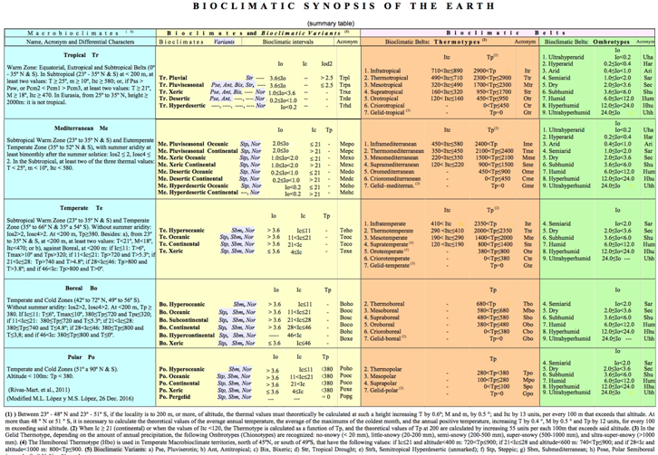
6.- ISOBIOCLIMATE
An Isobioclimate
is a unique bioclimatic space, defined by a Bioclimate / Variant, together with
a Bioclimatic Belt - Thermotype + Ombrotype-. Each Isobioclimate is an
elemental bioclimatic unit, as perceived and distinguished by living beings. We
can consider each Isobioclimate as a natural culture chamber, a Phytotron,
whose "walls" are the lower and upper thresholds that define each one
of its components: Macrobioclimate, Bioclimate / Variant and Bioclimatic
Belt-Thermotype and Ombrotype-. Considering fixed other environmental variables
- such as mother rock, soil, geological history, evolutionary history of living
beings, etc. - each Isobioclimate harbors, in a climax position, a single
vegetation series.
Isobioclimates
are useful for identifying bioclimatically analogous territories on any of the
five Continents, as well as for recognizing equivalent types of vegetation. The
representation on the map of the areas occupied by each Isobioclima allows very
precise bioclimatic maps to be obtained. (See figure 116, Isobioclimatic Map of
Peninsular Spain).
To name each
Isobioclimate is used a phrase that includes: Bioclimate / Bioclimatic Variant,
together with a Bioclimatic Belt - Thermotype + Ombrotype-. Thus, for example: Mepo Nor Tme Dry is the Isobioclimate "Mediterranean Pluviseasonal
Oceanic, Normal Variant, Thermomediterranean, Dry", which is found, for
example, in much of Andalusia, Spain; or Boxe
Stp Tbo Dry is the
Isobioclimate "Boreal Xeric Steppic, Termoboreal, Dry", which
operates, for example, in Petropavlovsk, Kazakhstan.
7.- BIOCLIMOGRAMS
Bioclimograms,
also called Bioclimographs, or Ombro-Termoclimograms, are the graphical
representation of Isobioclimates. Bioclimograms used by Rivas-Martínez (2008)
and Rivas-Martínez & al. (2011), are based on those of Gaussen &
Bagnouls (1952) and also on those of Walter & Lieth (1967). These graphs,
very expressive, represent, in a Cartesian coordinate system with two ordinates
and one abscissa, the temperature and rainfall data of a meteorological
station, throughout the year. In the left ordinate, the temperature is
represented, and in the right ordinate, the rainfall: their scales are adjusted
to the ratio 2T (ºC) = P (mm). On the abscissa, the months of the year are
represented: in the first place appears the month following the winter
solstice: January in the Northern Hemisphere, and July in the Southern
Hemisphere.
The graph of
Figure 8 is accompanied by a data panel, which includes:
name of the station
(1); its altitude in meters (2); its latitude, longitude, and the number of
years of meteorological observations (3); P (4), T (5), m (6), Ic
(7), M (8), Tp (9), Itc (10), Tn (11), Io (12); trimesterly precipitation in decreasing order (13): Pn=spring, S=summer,
F=automn, and W=winter; M
'(14); m' (15); temperature scale (16); precipitation scale (17).
Figure 8.- Structure of the Bioclimogram (Rivas-Mart,
2008, Rivas-Mart et al., 2011, somewhat modified by the authors). (Explanation
of numbers, in the text).
In order to
accommodate, in a single type of Bioclimograma, all the variations of Ti and Pi
occurring in the world, the temperature scale (16) starts at zero on the dotted
line and advances five degrees by five degrees above zero; with respect to
negative temperatures, the scale is modified and each interval represents the
following temperatures: -10, -20 y – 60ºC. As for the precipitations (17), each segment
represents 10mm of rainfall until reaching 90mm, because, from this rainfall,
the values are doubled for each interval: 180, 360 y 720mm of Pi
(18). The surface of
the rainfall curve, that exceeds the 90 mm line, is colored in blue (18) (in
this diagram we have put it in yellow), to indicate the change of scale. When
the temperature curve exceeds that of the precipitation, the area enclosed
between the two curves, drought expression (19), is colored red (in this scheme
we have put it in blue); But, if the rainfall curve exceeds that of the
temperature, that surface is striped, to indicate period with available
humidity (20). Monthly frost periods: sure or probable (21); and absent (22).
The period of plant activity, Pav, (23): months with Ti ≥ 3,5 °; NORTH HEMISPHERE: months in the Northern
Hemisphere, and HEMISPHERE SUR: months in the Southern Hemisphere: E, January;
...; X, July; ...; (24): at the bottom of the graph, the complete bioclimatic
diagnosis, the Isobioclimate, -including Macrobioclimate (named in the
Bioclimate), Bioclimate, Bioclimatic Variant and Bioclimatic Belt, expressed as
Thermotype and Ombrotype horizons-, is given.
8.- APPROACH to the GLOBAL BIOCLIMATIC DIVERSITY
Global
Bioclimatic Diversity can be considered at each of the three hierarchical
levels of the World Bioclimatic Classification:
8.1.-
At the first hierarchical level,
that of the Macrobioclimates, total
World Diversity is 5 Macrobioclimates.
8.2.- For the second hierarchical level, that of the Bioclimates/Variants, we have collected,
in figure 9, almost the whole totality of the World Diversity at this level, 74
Bioclimate / Variant units, distributed by Bioclimates and by Variants.
As for
Macrobioclimates, at this Bioclimate / Variant level, the most diversified is
the Tropical Macrobioclimate, with 18 Bioclimate/Variant units, followed by the
Boreal Macrobioclimate, with 17. By variants, the best represented are: the
Normal Variant, which is present in each Bioclimate, except in Tropical Pluvial
and Tropical Pluviseasonal; the Steppic Variant, present in 18 of the
Bioclimates; and the Submediterranean Variant, present in 15 Bioclimates.
8.3.- And, in the third hierarchical
level, that of the Bioclimatic Belts -Thermotypes and Ombrotypes-,the World Bioclimatic Diversity, at this level of Isobioclimates, is almost 400
Isobioclimates, although only about 300 Isobioclimates have a significant
territorial entity worldwide. (Rivas-Mart. & Rivas-Sáenz, 1996-2017;
Rivas-Mart. et al., 2011).
Figure 10 lists,
for each Macrobioclimate, the number of its Bioclimates, its Variants, its
combined units Bioclimate + Variant, and of the Thermotypes and Ombrotypes that
operate in it. And, in its last column, appears the approximate number of its
Isobioclimates
The world 's
largest bioclimatic diversity, at Isobioclimates level, is offered by Temperate
Macrobioclimate, with more than 97 Isobioclimates, followed by Tropical
Macrobioclimate, with more than 91.
Figure 9.- Almost all the
possible combinations of Bioclimate / Variant, in the 28 Bioclimates, of the
five Macrobioclimates, distributed by Bioclimates and by Variants.
|
Bioclimates |
Pse |
Ant |
Bix |
Str |
Stp |
Sbm |
Nor |
Total |
Total |
|
Trpl |
|
|
|
Pluvial Hygrophytic |
|
|
|
3 |
|
|
Pluvial Subhigrophytic |
|||||||||
|
Pluvial Submesophytic |
|||||||||
|
Trps |
• |
• |
• |
Pluviseasonal Mesophytic |
|
|
|
7 |
|
|
Pluviseasonal Submesophytic |
|||||||||
|
Pluviseasonal Subxerophytic |
|||||||||
|
Pluviseasonal Xerophytic |
|||||||||
|
Trxe |
• |
• |
• |
|
|
|
• |
4 |
|
|
Trde |
• |
• |
|
|
|
|
• |
3 |
|
|
Trhd |
|
|
|
|
|
|
• |
1 |
|
|
Total
Tropical |
|
|
|
|
|
|
|
|
18 |
|
Mepo |
|
|
|
|
• |
|
• |
2 |
|
|
Mepc |
|
|
|
|
• |
|
• |
2 |
|
|
Mexo |
|
|
|
|
• |
|
• |
2 |
|
|
Mexc |
|
|
|
|
• |
|
• |
2 |
|
|
Medo |
|
|
|
|
• |
|
• |
2 |
|
|
Medc |
|
|
|
|
• |
|
• |
2 |
|
|
Meho |
|
|
|
|
|
|
• |
1 |
|
|
Mehc |
|
|
|
|
|
|
• |
1 |
|
|
Total Mediterranean |
|
|
|
|
|
|
|
|
14 |
|
Teho |
|
|
|
|
|
• |
• |
2 |
|
|
Teoc |
|
|
|
|
• |
• |
• |
3 |
|
|
Teco |
|
|
|
|
• |
• |
• |
3 |
|
|
Texe |
|
|
|
|
• |
• |
• |
3 |
|
|
Total Temperate |
|
|
|
|
|
|
|
|
11 |
|
Boho |
|
|
|
|
|
• |
• |
2 |
|
|
Booc |
|
|
|
|
• |
• |
• |
3 |
|
|
Bosc |
|
|
|
|
• |
• |
• |
3 |
|
|
Boco |
|
|
|
|
• |
• |
• |
3 |
|
|
Bohc |
|
|
|
|
• |
• |
• |
3 |
|
|
Boxe |
|
|
|
|
• |
• |
• |
3 |
|
|
Total Boreal |
|
|
|
|
|
|
|
|
17 |
|
Poho |
|
|
|
|
|
• |
• |
2 |
|
|
Pooc |
|
|
|
|
• |
• |
• |
3 |
|
|
Poco |
|
|
|
|
• |
• |
• |
3 |
|
|
Poxe |
|
|
|
|
• |
• |
• |
3 |
|
|
Popg |
|
|
|
|
• |
• |
• |
3 |
|
|
Total Polar |
|
|
|
|
|
|
|
|
14 |
|
TOTAL |
3 |
3 |
2 |
7 |
18 |
15 |
26 |
74 |
74 |
Figure 10.- The almost
totality of World Bioclimatic Diversity at Isobioclimates level.
|
Macro-bioclimate |
Bio-climates |
Operating Variants |
Bioclimates + Variants |
Operating Thermo-types |
Operating Ombro-types |
Isobio-climates |
|
Tropical |
5 |
11 |
|
|
|
|
|
Mediterra-nean |
8 |
2 |
14 |
7 |
9 |
Más de 68 |
|
Temperate |
4 |
3 |
11 |
7 |
6 |
Más de 97 |
|
Boreal |
6 |
3 |
|
|
|
|
|
Polar |
5 |
3 |
|
|
|
|
|
Total |
28 |
13 in the world |
74 |
31 |
9 in the world |
Almost
400 |
8.4.-
As illustrative examples of World Bioclimatic Diversity, next we
give 59 climatic-bioclimatic examples, from as many meteorological stations,
which represent the majority of the existing combinations of Macrobioclimate, Bioclimate and Bioclimatic
Variant. Moreover, this information is available in: Worldwide Bioclimatic
Classification System, 1996-2017, S. Rivas-Martínez & S. Rivas-Sáenz,
Phytosociological Research Center, Spain, http://www.globalbioclimatics.org. In order to facilitate access to those examples, in
Figure 11 we give the list of the 59 selected stations, ordered according to
the Bioclimatic Synopsis of the Earth (see Figure 7, Chapter 5); and in figure
12, the list of those same selected stations, sorted alphabetically by country.
After the figures 11 and 12, appear each of the climatic-bioclimatic examples,
ordered by Bioclimate / Variant, figures 13-71.
Figure 11.- List of climate-bioclimatic
representative examples of almost every combination of Macrobioclimate and
Bioclimate / Bioclimatic Variant, with territorial representation on Earth, in
bioclimatic order.
|
|
Bioclimate / Variant |
Country |
Weather Station |
|
1 |
Trpl Hygrophytic |
Japan |
Ishigaki |
|
2 |
Trpl
Subhigrophytic |
Suriname |
Zanderij |
|
3 |
Trpl
Submesophytic |
China |
Wucho/Tsang-Wu |
|
4 |
Trps
Mesophytic |
Indonesia |
Achmad Yani |
|
5 |
Trps
Submesophytic |
Bahamas Islands |
Nassau
Intl |
|
6 |
Trps
Subxerophytic |
Madagascar |
Tananarive |
|
7 |
Trps Xerophytic |
Mexico |
Zapopán |
|
8 |
Trps Pse |
Vietnam |
Donghoi |
|
9 |
Trps Ant |
Sri Lanka |
Trincomalee |
|
10 |
Trps Bix |
Ivory Coast |
Port Bouet |
|
11 |
Trxe Pse |
Chad |
Ati |
|
12 |
Trxe Ant |
Saudi Arabia |
Khamis Mushait |
|
13 |
Trxe Bix |
Ethiopia |
Diredawa |
|
14 |
Trxe Normal |
Botswana |
Ghanzi |
|
15 |
Trde Pse |
Peru |
Arequipa |
|
16 |
Trde Ant |
Iran |
Jask |
|
17 |
Trde Normal |
Pakistan |
Karachi |
|
18 |
Trhd Normal |
Namibia |
Mowebaai |
|
19 |
Mepo Stp |
Spain |
Tudela |
|
20 |
Mepo Normal |
Chile |
Hualpencillo |
|
21 |
Mepc Stp |
Ukraine |
Bolgrad |
|
22 |
Mepc Normal |
Tajikistan |
Dushanbe |
|
23 |
Mexo Stp |
Argentina |
Coronel J.J.Gómez |
|
24 |
Mexo Normal |
Libya |
Idris |
|
25 |
Mexc
Stp |
Kazakhstan |
Pavlodar |
|
26 |
Mexc
Normal |
Armenia |
Jerevan |
|
27 |
Medo
Stp |
Australia |
Farina |
|
28 |
Medo
Normal |
Egypt |
Salum |
|
29 |
Medc
Stp |
Kazakhstan |
Dzhezkazgan |
|
30 |
Medc
Normal |
Uzbekistan |
Ak-Baytal |
|
31 |
Meho
Normal |
Libya |
Gialo |
|
32 |
Mehc
Normal |
Iran |
Yazd |
|
33 |
Teho
Sbm |
New Zealand |
Wigram |
|
34 |
Teho
Normal |
Ireland |
Valentia |
|
35 |
Teoc
Stp |
China |
Matsu |
|
36 |
Teoc
Sbm |
Croatia |
Rab |
|
37 |
Teoc
Normal |
Uruguay |
Artigas |
|
38 |
Teco
Stp |
Hungary |
Pecs |
|
39 |
Teco
Sbm |
India |
Srinagar |
|
40 |
Teco
Normal |
Byelarus |
Brest |
|
41 |
Texe
Stp |
Mongolia |
Altai |
|
42 |
Texe
Sbm |
Ukraine |
Kharkov |
|
43 |
Texe
Normal |
Argentina |
Villa Mercedes |
|
44 |
Boho
Normal |
Chile |
Navarino |
|
45 |
Booc
Normal |
Iceland |
Husavik |
|
46 |
Bosc
Stp |
Sweden |
Bjuroklubb |
|
47 |
Bosc
Normal |
Finland |
Oulu |
|
48 |
Boco
Stp |
Russia |
Anavgay Kamchatk |
|
49 |
Boco
Normal |
Mongolia |
Bulgan |
|
50 |
Bohc
Stp |
Russia Yakutskaya |
Verkhoyansk |
|
51 |
Bohc
Normal |
Russia Yakutskaya |
Komara |
|
52 |
Boxe
Stp |
USA Alaska |
Fort Yukon |
|
53 |
Poho
Normal |
Norway |
Jan Mayen |
|
54 |
Pooc
Normal |
Greenland -DNK- |
Ivigtut |
|
55 |
Poco
Stp |
Canada |
Cambridge Bay |
|
56 |
Poco
Normal |
Russia |
Yamsk |
|
57 |
Poxe
Stp |
Russia Yakutia |
Sredne-Kolymsk |
|
58 |
Poxe
Normal |
Greenland-Dnk |
Umanak |
|
59 |
Popg
Normal |
Antarctica |
Mcmurdo Station |
Figure 12.- List
of climate-bioclimatic representative examples of almost every combination of Macrobioclimate
and Bioclimate / Bioclimatic Variant, with territorial representation on Earth, in alphabetical order
of countries.
|
|
Country |
Weather Station |
Bioclimate/ Variant |
|
59 |
Antarctica |
Mcmurdo Station |
Popg
Normal |
|
23 |
Argentina |
Coronel J.J. Gómez |
Mexo Stp |
|
43 |
Argentina |
Villa Mercedes |
Texe
Normal |
|
26 |
Armenia |
Jerevan |
Mexc
Normal |
|
27 |
Australia |
Farina |
Medo
Stp |
|
5 |
Bahamas Islands |
Nassau Intl |
Trps Submesophytic |
|
14 |
Botswana |
Ghanzi |
Trxe Normal |
|
40 |
Byelarus |
Brest |
Teco
Normal |
|
55 |
Canada |
Cambridge Bay |
Poco
Stp |
|
11 |
Chad |
Ati |
Trxe Pse |
|
20 |
Chile |
Hualpencillo |
Mepo Normal |
|
44 |
Chile |
Navarino |
Boho
Normal |
|
3 |
China |
Wucho/Tsang-Wu |
Trpl
Submesophytic |
|
35 |
China |
Matsu |
Teoc
Stp |
|
36 |
Croatia |
Rab |
Teoc
Sbm |
|
28 |
Egypt |
Salum |
Medo
Normal |
|
13 |
Ethiopia |
Diredawa |
Trxe Bix |
|
47 |
Finland |
Oulu |
Bosc
Normal |
|
54 |
Greenland -DNK- |
Ivigtut |
Pooc
Normal |
|
58 |
Greenland-Dnk |
Umanak |
Poxe
Normal |
|
38 |
Hungary |
Pecs |
Teco
Stp |
|
45 |
Iceland |
Husavik |
Booc
Normal |
|
39 |
India |
Srinagar |
Teco
Sbm |
|
4 |
Indonesia |
Achmad Yani |
Trps
Mesophytic |
|
16 |
Iran |
Jask |
Trde Ant |
|
32 |
Iran |
Yazd |
Mehc
Normal |
|
34 |
Ireland |
Valentia |
Teho
Normal |
|
10 |
Ivory Coast |
Port Bouet |
Trps Bix |
|
1 |
Japan |
Ishigaki |
Trpl Hygrophytic |
|
25 |
Kazakhstan |
Pavlodar |
Mexc
Stp |
|
29 |
Kazakhstan |
Dzhezkazgan |
Medc
Stp |
|
24 |
Libya |
Idris |
Mexo Normal |
|
31 |
Libya |
Gialo |
Meho
Normal |
|
6 |
Madagascar |
Tananarive |
Trps
Subxerophytic |
|
7 |
Mexico |
Zapopán |
Trps Xerophytic |
|
41 |
Mongolia |
Altai |
Texe
Stp |
|
49 |
Mongolia |
Bulgan |
Boco
Normal |
|
18 |
Namibia |
Mowebaai |
Trhd Normal |
|
33 |
New Zealand |
Wigram |
Teho
Sbm |
|
53 |
Norway |
Jan Mayen |
Poho
Normal |
|
17 |
Pakistan |
Karachi |
Trde Normal |
|
15 |
Peru |
Arequipa |
Trde Pse |
|
48 |
Russia |
Anavgay Kamchatk |
Boco
Stp |
|
56 |
Russia |
Yamsk |
Poco
Normal |
|
57 |
Russia Yakutia |
Sredne-Kolymsk |
Poxe
Stp |
|
50 |
Russia Yakutskaya |
Verkhoyansk |
Bohc
Stp |
|
51 |
Russia Yakutskaya |
Komara |
Bohc
Normal |
|
12 |
Saudi Arabia |
Khamis Mushait |
Trxe Ant |
|
19 |
Spain |
Tudela |
Mepo Stp |
|
9 |
Sri Lanka |
Trincomalee |
Trps Ant |
|
2 |
Suriname |
Zanderij |
Trpl
Subhigrophytic |
|
46 |
Sweden |
Bjuroklubb |
Bosc
Stp |
|
22 |
Tajikistan |
Dushanbe |
Mepc Normal |
|
21 |
Ukraine |
Bolgrad |
Mepc Stp |
|
42 |
Ukraine |
Kharkov |
Texe
Sbm |
|
37 |
Uruguay |
Artigas |
Teoc
Normal |
|
52 |
USA Alaska |
Fort Yukon |
Boxe
Stp |
|
30 |
Uzbekistan |
Ak-Baytal |
Medc
Normal |
|
8 |
Vietnam |
Donghoi |
Trps Pse |
Next, the 59
stations, as examples of the bioclimatic diversity at the level of
Macrobioclima - Bioclima / Variant, ordered by that concept, following figure
11.
Note: At the computer exits,
from the web http://www.globalbioclimatics.org, the stations in which
no variant is specified, must be considered as Normal Variant (Nor) (See Normal
Variant, above). We add this indication in each of the stations with Variante
Nor.
Figure 13
|
|
01 |
|
|
|
|
|
|
|
Tropical
Pluvial Bioclimate, Hygrophytic Variant |
|
Figure 14
|
|
02 |
|
|
|
|
|
|
|
Tropical
Pluvial Bioclimate, Subhigrophytic
Variant |
|
Figure 15
|
|
03 |
|
|
|
|
|
|
|
Tropical
Pluvial Bioclimate, Submesophytic Variant |
|

Figure 16
|
|
04 |
|
|
|
|
|
|
|
Tropical Pluviseasonal Bioclimate, Mesophytic Variant |
|
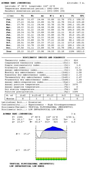
Figure 17
|
|
05 |
|
|
|
|
|
|
|
Tropical Pluviseasonal Bioclimate, Submesophytic Variant |
|
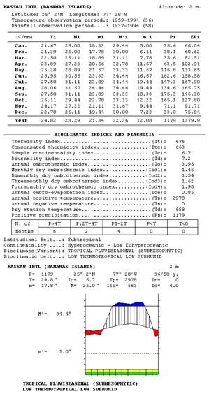
Figure 18
|
|
06 |
|
|
|
|
|
|
|
Tropical Pluviseasonal Bioclimate, Subxerophytic Variant |
|
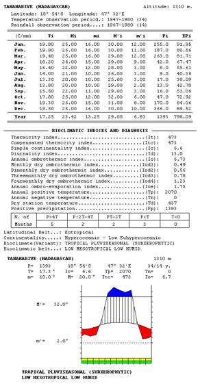
Figure 19
|
|
07 |
|
|
|
|
|
|
|
Tropical Pluviseasonal Bioclimate, Xerophytic Variant |
|
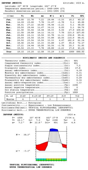
Figure 20
|
|
08 |
|
|
|
|
|
|
|
Tropical
Pluviseasonal Bioclimate, Pluviserotin Variant |
|
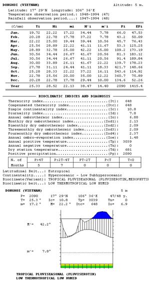
Figure 21
|
|
09 |
|
|
|
|
|
|
|
Tropical
Pluviseasonal Bioclimate, Antitropical Variant |
|
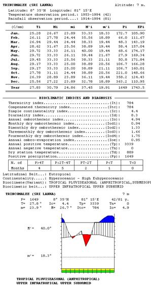
Figure 22
|
|
10 |
|
|
|
|
|
|
|
Tropical Pluviseasonal Bioclimate, Bixeric Variant |
|
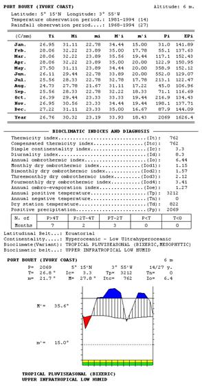
Figure
23
|
|
11 |
|
|
|
|
|
|
|
Tropical
Xeric Bioclimate, Pluviserotin Variant |
|
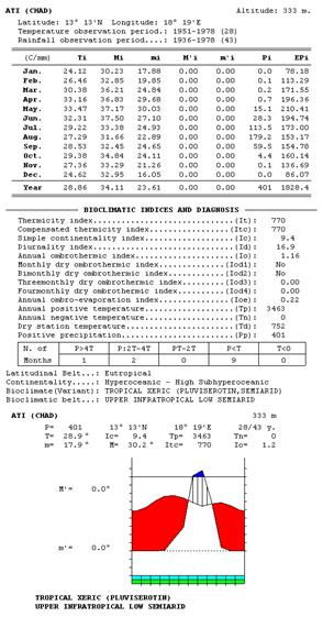
Figure 24
|
|
12 |
|
|
|
|
|
|
|
Tropical
Xeric Bioclimate, Antitropical Variant |
|
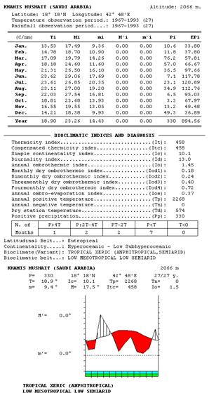
Figure 25
|
|
13 |
|
|
|
|
|
|
|
Tropical Xeric Bioclimate,
Bixeric Variant |
|
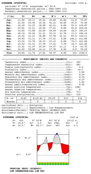
Figure 26
|
|
14 |
|
|
|
|
|
|
|
Tropical
Xeric Bioclimate, Normal Variant |
|
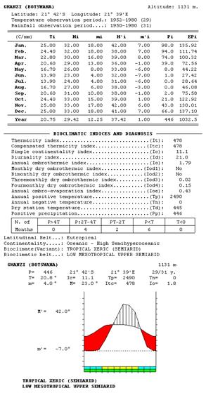
Figure 27
|
|
15 |
|
|
|
|
|
|
|
Tropical
Desertic Bioclimate, Pluviserotin Variant |
|
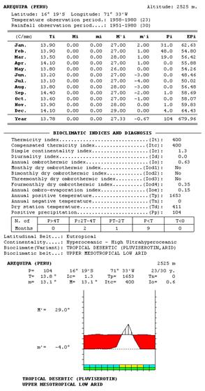
Figure 28
|
|
16 |
|
|
|
|
|
|
|
Tropical
Desertic Bioclimate, Antitropical Variant |
|
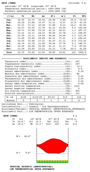
Figure 29
|
|
17 |
|
|
|
|
|
|
|
Tropical
Desertic Bioclimate, Normal Variant |
|
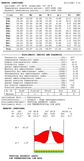
Figure 30
|
|
18 |
|
|
|
|
|
|
|
Tropical
Hyperdesertic Bioclimate, Normal Variant |
|
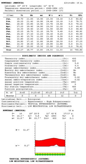
Figure 31
|
|
19 |
|
|
|
|
|
|
|
Mediterranean Pluviseasonal Oceanic Bioclimate, Steppic Variant |
|
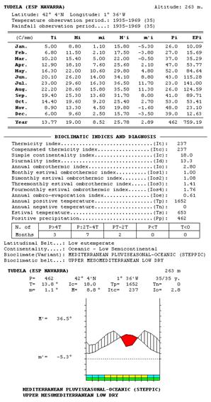
Figure 32
|
|
20 |
|
|
|
|
|
|
|
Mediterranean
Pluviseasonal Oceanic Bioclimate,
Normal Variant |
|
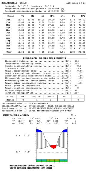
Figure 33
|
|
21 |
|
|
|
|
|
|
|
Mediterranean Pluviseasonal Continental
Bioclimate, Steppic Variant |
|
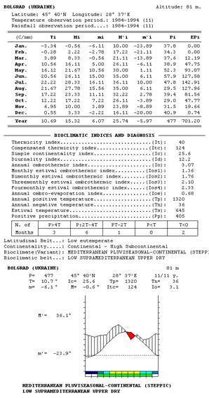
Figure 34
|
|
22 |
|
|
|
|
|
|
|
Mediterranean Pluviseasonal Continental Bioclimate, Steppic
Variant |
|
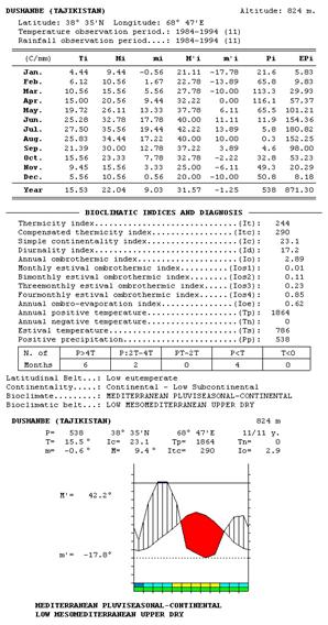
Figure 35
|
|
23 |
|
|
|
|
|
|
|
Mediterranean Xeric Oceanic Bioclimate, Steppic Variant |
|
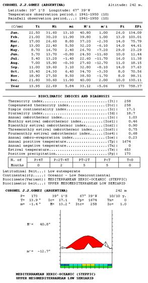
Figure 36
|
|
24 |
|
|
|
|
|
|
|
Mediterranean
Xeric Oceanic Bioclimate,
Normal Variant |
|
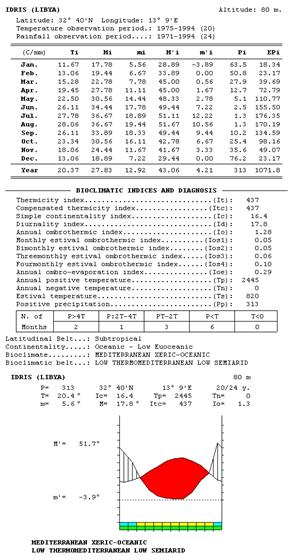
Figure 37
|
|
25 |
|
|
|
|
|
|
|
Mediterranean Xeric Continental Bioclimate, Steppic Variant |
|
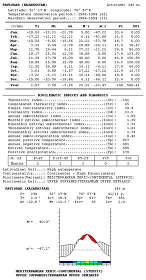
Figure 38
|
|
26 |
|
|
|
|
|
|
|
Mediterranean
Xeric Continental Bioclimate,
Normal Variant |
|
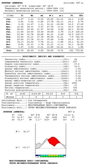
Figure 39
|
|
27 |
|
|
|
|
|
|
|
Mediterranean Desertic Oceanic Bioclimate, Steppic Variant |
|
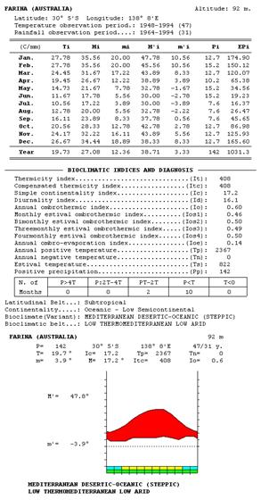
Figure 40
|
|
28 |
|
|
|
|
|
|
|
Mediterranean
Desertic Oceanic Bioclimate,
Normal Variant |
|
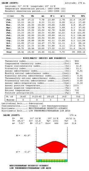
Figure 41
|
|
29 |
|
|
|
|
|
|
|
Mediterranean Desertic Continental Bioclimate, Steppic Variant |
|
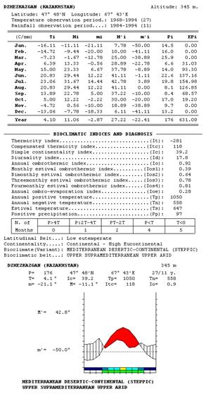
Figure 42
|
|
30 |
|
|
|
|
|
|
|
Mediterranean
Desertic Continental Bioclimate,
Normal Variant |
|
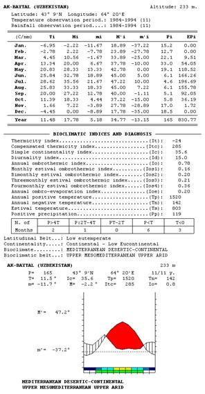
Figure 43
|
|
31 |
|
|
|
|
|
|
|
Mediterranean
Hyperdesertic Oceanic Bioclimate,
Normal Variant |
|
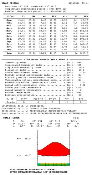
Figure 44
|
|
32 |
|
|
|
|
|
|
|
Mediterranean
Hyperdesertic Continental Bioclimate, Normal Variant |
|
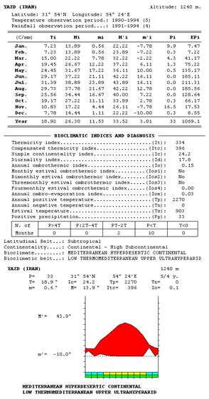
Figure 45
|
|
33 |
|
|
|
|
|
|
|
Temperate
Hyperoceanic Bioclimate,
Submediterranean Variant |
|
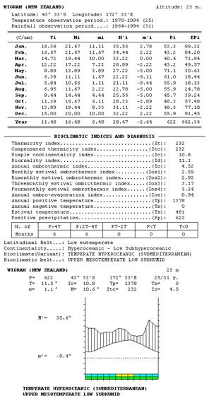
Figure 46
|
|
34 |
|
|
|
|
|
|
|
Temperate
Hyperoceanic Bioclimate,
Normal Variant |
|
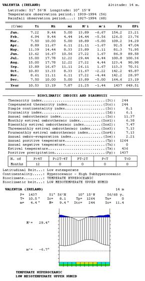
Figure 47
|
|
35 |
|
|
|
|
|
|
|
Temperate Oceanic Bioclimate, Steppic Variant |
|
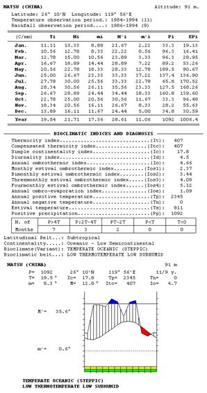
Figure 48
|
|
36 |
|
|
|
|
|
|
|
Temperate
Oceanic Bioclimate,
Submediterranean Variant |
|
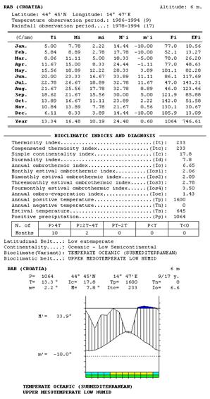
Figure 49
|
|
37 |
|
|
|
|
|
|
|
Temperate Oceanic Bioclimate, Normal Variant |
|
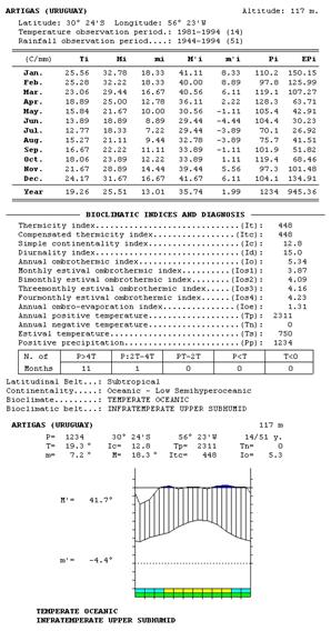
Figure 50
|
|
38 |
|
|
|
|
|
|
|
Temperate Continental Bioclimate, Steppic Variant |
|
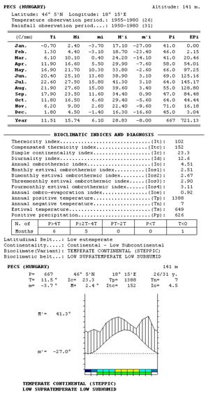
Figure 51
|
|
39 |
|
|
|
|
|
|
|
Temperate
Continental Bioclimate,
Submediterranean Variant |
|
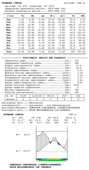
Figure 52
|
|
40 |
|
|
|
|
|
|
|
Temperate
Continental Bioclimate,
Normal Variant |
|
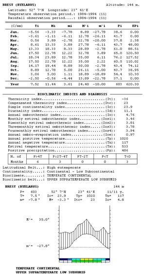
Figure 53
|
|
41 |
|
|
|
|
|
|
|
Temperate Xeric Bioclimate, Steppic Variant |
|
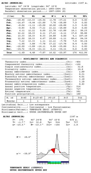
Figure 54
|
|
42 |
|
|
|
|
|
|
|
Temperate
Xeric Bioclimate,
Submediterranean Variant |
|
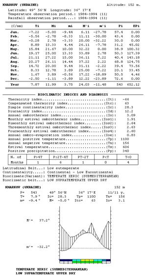
Figure 55
|
|
43 |
|
|
|
|
|
|
|
Temperate
Xeric Bioclimate,
Normal Variant |
|
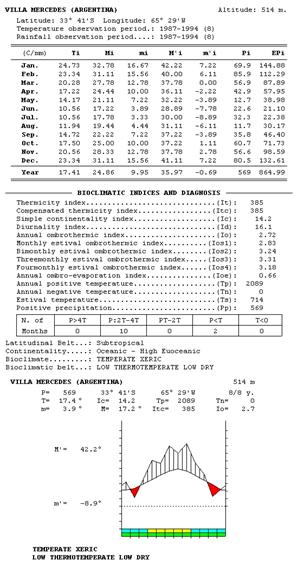
Figure 56
|
|
44 |
|
|
|
|
|
|
|
Boreal
Hyperoceanic Bioclimate,
Normal Variant |
|
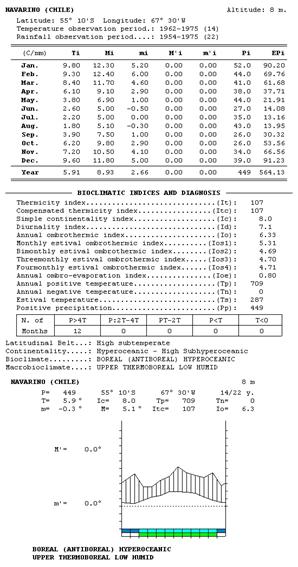
Figure 57
|
|
45 |
|
|
|
|
|
|
|
Boreal
Oceanic Bioclimate,
Normal Variant |
|
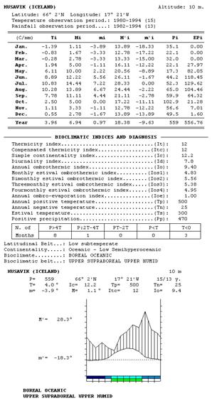
Figure 58
|
|
46 |
|
|
|
|
|
|
|
Boreal Subcontinental Bioclimate, Steppic Variant |
|
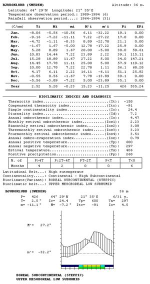
Figure 59
|
|
47 |
|
|
|
|
|
|
|
Boreal
Subcontinental Bioclimate,
Normal Variant |
|
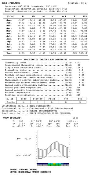
Figure 60
|
|
48 |
|
|
|
|
|
|
|
Boreal Continental Bioclimate, Steppic Variant |
|
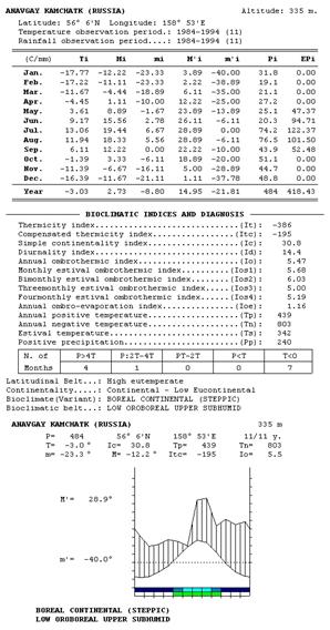
Figure 61
|
|
49 |
|
|
|
|
|
|
|
Boreal
Continental Bioclimate, Normal Variant |
|
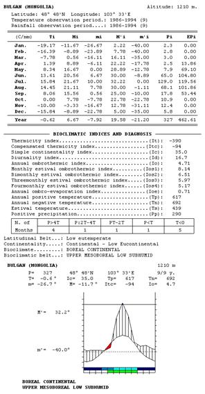
Figure 62
|
|
50 |
|
|
|
|
|
|
|
Boreal Hypercontinental Bioclimate, Steppic Variant |
|
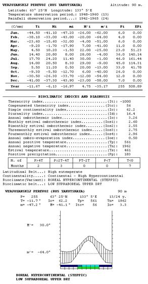
Figure 63
|
|
51 |
|
|
|
|
|
|
|
Boreal
Hypercontinental Bioclimate,
Normal Variant |
|
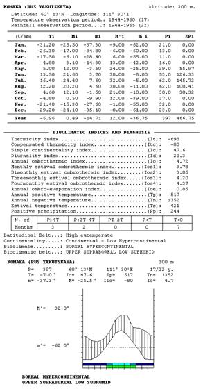
Figure 64
|
|
52 |
|
|
|
|
|
|
|
Boreal
Hypercontinental Bioclimate,
Normal Variant |
|
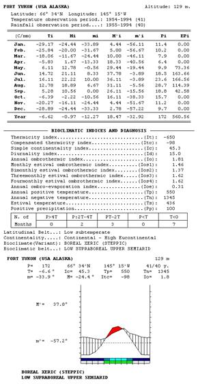
Figure 65
|
|
53 |
|
|
|
|
|
|
|
Polar
Hyperoceanic Bioclimate,
Normal Variant |
|
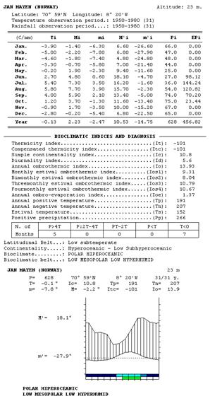
Figure 66
|
|
54 |
|
|
|
|
|
|
|
Polar Oceanic Bioclimate, Normal Variant |
|
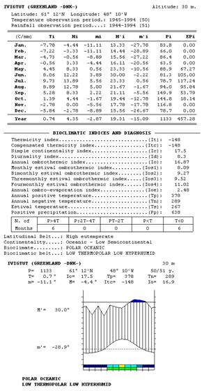
Figure 67
|
|
55 |
|
|
|
|
|
|
|
Polar Continental Bioclimate, Steppic Variant |
|
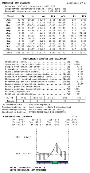
Figure 68
|
|
56 |
|
|
|
|
|
|
|
Polar
Continental Bioclimate,
Normal Variant |
|
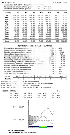
Figure 69
|
|
57 |
|
|
|
|
|
|
|
Polar Xeric Bioclimate, Steppic Variant |
|
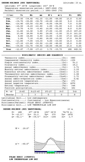
Figure 70
|
|
58 |
|
|
|
|
|
|
|
Polar
Xeric Bioclimate,
Normal Variant |
|
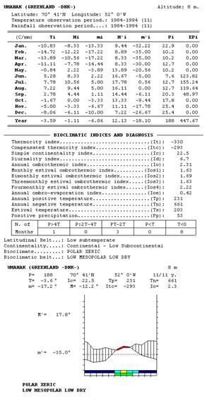
Figure 71
|
|
59 |
|
|
|
|
|
|
|
Polar
Pergelid Bioclimate,
Normal Variant |
|
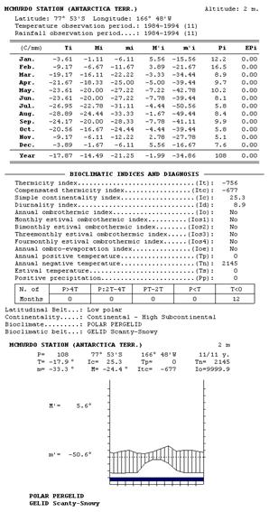
9.- ASSESSMENT OF SUMMER ARIDITY, WITH EXAMPLES
Summer aridity, Ios2 ≤ 2 (see Chapter 3, Ombrothermal Indexes, and Chapter 4,
Mediterranean, Temperate and Boreal Macrobioclimates), differentiates the
Mediterranean Macrobioclimate from the Temperate and Boreal Macrobioclimates,
which do not have such summer aridity. However, there are circumstances where
the soil field capacity supplements this summer aridity, If the month, or the
two months, prior to the summer drought, provide enough rain, to have the soil
recharged: in those cases, neither the vegetation nor the Macrobioclimate are
Mediterranean. In order to evaluate this possible soil compensation for summer
aridity, Summer Compensatory Ombrothermal Indexes, Iosc3 e Iosc4, are used (see Chapter 3). The values of these
Compensable Summer Ombrothermal Indices, Iosc3 e Iosc4, have a high discriminatory value in the
Mediterranean-Temperate and Mediterranean-Boreal border territories.
9.1.- Assessment of summer aridity.
From what has
been said, if the Ios2 of our weather station is less than or equal to 2, Ios2 ≤ 2, we can not categorically state that our weather
station has summer aridity, but we must study the possible edaphic compensation
to this summer aridity, with the help of Iosc3 and Iosc4 values. However, the possible compensatory effect of precipitation
falling in the month, or in the two months preceding the summer drought, is
related to three factors: a), the annual water comfort, measured by the annual Io; b), the magnitude of Ios2; and c), the own value of the compensable
Ombrothermal Indices, Iosc3 and Iosc4. Which is understandable: Not any value of Io allows the compensation, but this can only occur with
an Io annual
greater than 2. But, in addition, and depending on the magnitude of the annual Io, the possibly compensable values of Ios2 vary. In figures 72 and 73, the values of Io and Ios2, which allow for compensation, are given. If our weather station allows
the compensation of a deficient Ios2, three cases may occur: 1), that our Iosc3 value were greater than two, which would suppose
directly that the summer aridity is compensated, that is to say, there is no
summer aridity; 2), that our Iosc3 value were below the corresponding intervals in the
table, which would indicate, directly, that there is no compensation to summer
aridity; and 3), that our Iosc3 value were in between the intervals shown in the table
to allow compensation with Iosc4. Already in the column of Iosc4, there are only two possibilities: 1), that our Iosc4 were greater than two, which indicates that there is
edaphic compensation of summer aridity; and 2), that our Iosc4 were less than or equal to 2, which finally indicates
that there is no edaphic compensation of summer aridity. (The reading and
interpretation of Figure 72 is explained in Figure 73).
Figure 72.- Compensation
table to evaluate summer aridity, as a function of Io, Ios2, Iosc3 and Iosc4.
|
Io |
|
|
Iosc4 |
|
2.0 < Io ≤ 2.8 |
|
|
- Iosc4
> 2.0: Compensable aridity - Iosc4 ≤
2.0: Non-compensable aridi |
|
2.8 < Io ≤ 3.6 |
1.8 ≤ Ios2 ≤ 2.0 |
1.9 ≤ Iosc3 ≤ 2.0 |
|
|
3.6 < Io ≤ 4.8 |
1.8 ≤ Ios2 ≤ 2.0 |
1.9 ≤ Iosc3 ≤ 2.0 |
|
|
4.8 < Io ≤ 6.0 |
|
|
|
|
6.0 < Io ≤ 7.0 |
|
|
|
|
7.0 < Io ≤ 8.0 |
1.4 ≤ Ios2 ≤ 2.0 |
1.8 ≤ Iosc3 ≤ 2.0 |
|
|
8.0 < Io ≤ 9.0 |
|
|
|
|
9.0 < Io ≤ 10.0 |
1.2 ≤ Ios2 ≤ 2.0 |
1.8 ≤ Iosc3 ≤ 2.0 |
|
|
10.0 < Io ≤ 11.0 |
1.1 ≤ Ios2 ≤ 2.0 |
1.7 ≤ Iosc3 ≤ 2.0 |
|
|
11.0 < Io ≤ 12.0 |
1.0 ≤ Ios2 ≤ 2.0 |
1.7 ≤ Iosc3 ≤ 2.0 |
|
|
12.0 < Ioaaaaa |
0.9 ≤ Ios2 ≤ 2.0 |
1.7 ≤ Iosc3 ≤ 2.0 |
Figure 73: Reading and
interpretation of figure 72.
|
Io |
|
Iosc3 |
|
|
2.0 < Io ≤
2.8 |
With Ios2 from 1.9 to 2.0, the
meteorological station is compensable
with Iosc3 If Ios2 is less than 1.9, the meteorological station is Mediterranean |
If Iosc3 is higher than 2.0, the weather station is Temperate, or Boreal If Iosc3 equals 2.0, the weather station
is compensable with Iosc4 If Iosc3 is less than 2.0, the meteorological station is Mediterranean |
If Iosc4 is greater than 2.0, the weather station is Tempe-rate, or Boreal If Iosc4 is less than or equal to 2.0, the weather station is Mediterranean |
|
2.8 < Io ≤
3.6 |
With Ios2 from 1.8 to 2.0, the
meteorological station is compensable
with Iosc3 If Ios2 is less than 1.8, the meteorological stationis Mediterranean |
If Iosc3 is higher than 2.0, the weather station is Temperate, or Boreal If Iosc3 goes from 1.9 to 2.0, the weather station is compensable with Iosc4 If Iosc3 is less than 1.9, the meteorological station is Mediterranean |
If Iosc4 is greater than 2.0, the weather station is Tempe-rate, or Boreal If Iosc4 is less than or equal to 2.0, the weather station is Mediterranean |
|
3.6 < Io ≤
4.8 |
With Ios2 from 1.8 to 2.0, the
meteorological station is compensable
with Iosc3 If Ios2 is less than 1.8, the meteorological station is Mediterranean |
If Iosc3 is higher than 2.0, the weather station is Temperate, or Boreal If Iosc3 goes from 1.9 to 2.0, the weather station is compensable with Iosc4 If Iosc3 is less than 1.9, the meteorological station is Mediterranean |
If Iosc4 is greater than 2.0, the weather station is Temperate, or Boreal If Iosc4 is less than or equal to 2.0, the weather station is Mediterranean |
|
4.8 < Io ≤
6.0 |
With Ios2 from 1.7 to 2.0, the
meteorological station is compensable
with Iosc3 If Ios2 is less than 1.7, the meteorological station is Mediterranean |
If Iosc3 is higher than 2.0, the weather station is Temperate, or Boreal If Iosc3 goes from 1.9 to 2.0, the weather station is compensable with Iosc4 If Iosc3 is less than 1.9, the meteorological station is Mediterranean |
If Iosc4 is greater than 2.0, the weather station is Temperate, or Boreal If Iosc4 is less than or equal to 2.0, the weather station is Mediterranean |
|
6.0 < Io ≤
7.0 |
With Ios2 from 1.5 to 2.0, the
meteorological station is compensable
with Iosc3 If Ios2 is less than 1.5, the meteorological station is Mediterranean |
If Iosc3 is higher than 2.0, the weather station is Temperate, or Boreal If Iosc3 goes from 1.8 to 2.0, the weather station is compensable with Iosc4 If Iosc3 is less than 1.8, the meteorological station is Mediterranean |
If Iosc4 is greater than 2.0, the weather station is Temperate, or Boreal If Iosc4 is less than or equal to 2.0, the weather station is Mediterranean |
|
7.0 < Io ≤
8.0 |
With Ios2 from 1.4 to 2.0, the
meteorological station is compensable
with Iosc3 If Ios2 is less than 1.4, the meteorological station is Mediterranean |
If Iosc3 is higher than 2.0, the weather station is Temperate, or Boreal If Iosc3 goes from 1.8 to 2.0, the weather station is compensable with Iosc4 If Iosc3 is less than 1.8, the meteorological station is Mediterranean |
If Iosc4 is greater than 2.0, the weather station is Temperate, or Boreal If Iosc4 is less than or equal to 2.0, the weather station is Mediterranean |
|
8.0 < Io ≤
9.0 |
With Ios2 from 1.3 to 2.0, the
meteorological station is compensable
with Iosc3 If Ios2 is less than 1.3, the meteorological station is Mediterranean |
If Iosc3 is higher than 2.0, the weather station is Temperate, or Boreal If Iosc3 goes from 1.8 to 2.0, the weather station is compensable with Iosc4 If Iosc3 is less than 1.8, the meteorological station is Mediterranean |
If Iosc4 is greater than 2.0, the weather station is Temperate, or Boreal If Iosc4 is less than or equal to 2.0, the weather station is Mediterranean |
|
9.0 < Io ≤10.0
|
With Ios2 from 1.2 to 2.0, the
meteorological station is compensable
with Iosc3 If Ios2 is less than 1.2, the meteorological station is Mediterranean |
If Iosc3 is higher than 2.0, the weather station is Temperate, or Boreal If Iosc3 goes from 1.8 to 2.0, the weather station is compensable with Iosc4 If Iosc3 is less than 1.8, the meteorological station is Mediterranean |
If Iosc4 is greater than 2.0, the weather station is Temperate, or Boreal If Iosc4 is less than or equal to 2.0, the weather station is Mediterranean |
|
10.0< Io ≤11.0
|
With Ios2 from 1.1 to 2.0, the
meteorological station is compensable
with Iosc3 If Ios2 is less than 1.1, the meteorological station is Mediterranean |
If Iosc3 is higher than 2.0, the weather station is Temperate, or Boreal If Iosc3 goes from 1.7 to 2.0, the weather station is compensable with Iosc4 If Iosc3 is less than 1.7, the meteorological station is Mediterranean |
If Iosc4 is greater than 2.0, the weather station is Temperate, or Boreal If Iosc4 is less than or equal to 2.0, the weather station is Mediterranean |
|
|
With Ios2 from 1.0 to 2.0, the
meteorological station is compensable
with Iosc3 If Ios2 is less than 1.0, the meteorological station is Mediterranean |
If Iosc3 is higher than 2.0, the weather station is Temperate, or Boreal If Iosc3 goes from 1.7 to 2.0, the weather station is compensable with Iosc4 If Iosc3 is less than 1.7, the meteorological station is Mediterranean |
If Iosc4 is greater than 2.0, the weather station is Temperate, or Boreal If Iosc4 is less than or equal to 2.0, the weather station is Mediterranean |
|
12.0 < Io |
With Ios2 from 0.9 to 2.0, the
meteorological station is compensable
with Iosc3 If Ios2 is less than 0.9, the meteorological station is Mediterranean |
If Iosc3 is higher than 2.0, the weather station is Temperate, or Boreal If Iosc3 goes from 1.7 to 2.0, the weather station is compensable with Iosc4 If Iosc3 is less than 1.7, the meteorological station is Mediterranean |
If Iosc4 is greater than 2.0, the weather station is Temperate, or Boreal If Iosc4 is less than or equal to 2.0, the weather station is Mediterranean |
9.2.- Examples for the valuation of summer aridity
Using the tables
in figures 72 and 73, the possible compensation of the summer aridity, Ios2 ≤ 2, is evaluated, analyzing the values of Io, Ios2, Iosc3 and Iosc4. To explain the use of the compensation tables, we
will use figures 74-79, whose information is taken from Rivas Martínez website:
www.globalbioclimatics.org.
The possible
edaphic compensation of the summer aridity has to be evaluated only when the Ios2 of our station is between 2 and 0.9, 0.9≤ Ios2 ≤
2, because if the station's Ios2 is greater than two (Ios2 > 2), the station has no summer aridity, and does not need
any compensation (figure 74): Smithers, Canada; however, if the station's Ios2 is less than 0.9, Ios2 <0.9, the station, with such a low Ios2, does not allow compensation for summer aridity
(figure 75: Dzhalal-Abad, Kyrgyzstan); but if the station's Ios2 is greater than or equal to 0.9, and equal to or less
than two: 0.9 ≤ Ios2 ≤ 2, the
existing summer aridity may, or may not, be compensable, and in order to
elucidate it, one must go again to the two tables in Figures 72 and 73, that
show how a deficient Ios2 can be compensated according to the value of the
annual Io, the Ios2 itself, and the Iosc3 and Iosc4. (See Figures 76 and 78, non-compensable, and figures
77 and 79, compensable).
Procedure:
Specifically, in order to analyze the possible edaphic compensation of summer
aridity, we look at the first column of Figures 72 and 73, to locate in which
interval of their first columns is our Io, and to work, then, on that row.
Already in the Ios2 column, two
things can happen: or that our Ios2 is less than the indicated interval, which would
automatically qualify the station as summer arid, without possible compensation
(figure 76: Skopje, Macedonia); or that our Ios2 is included in the indicated interval, which allows to
try the compensation with Iosc3. Then we go to the Iosc3 column: if our Iosc3 is greater than two, the summer aridity is compensated
(figure 77: Alustante, Guadalajara, Spain); if our Iosc3 is less than the indicated interval, the summer
aridity is definitely not compensable (Figure 78: Pounds Field, Texas); but if
our Iosc3 is within
the indicated range, the summer aridity can still be compensated with the Iosc4. In the Iosc4 column, two things can happen: or that our Iosc4 is greater than two, which indicates that summer
aridity is compensated by edaphic moisture (Figure 79: Atlanta, Georgia, USA);
or that our Iosc4 is equal to or less than two, indicating that the summer
aridity would be, definitely, not compensable (we have not found on the website
of Rivas Martínez, www.globalbioclimatics.org, any station of these
characteristics).
As we have said
above, the values of the Ombrothermic Indexes used in the compensation - Iosc3 and Iosc4 -, have a high discriminatory value in the
Mediterranean-Temperate and Mediterranean-Boreal border territories.
Figure 74
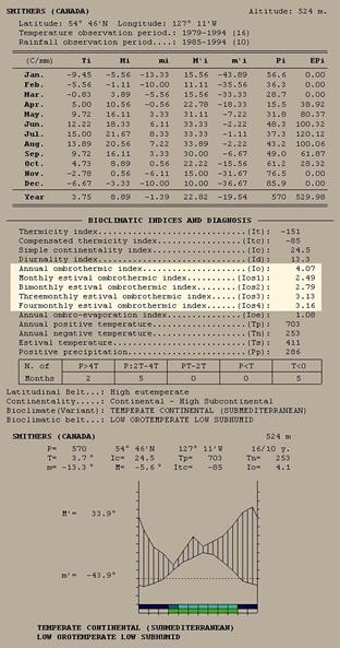
Bioclimatic
Diagnosis: Temperate Continental
Bioclimate,
Submediterranean
Variant
Figure 75
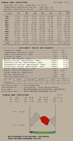
Diagnosis
Bioclimática: Mediterráneo Pluviestacional Continental,
Variante
NORMAL
Figure 76
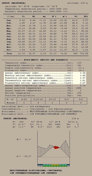
Bioclimatic
Diagnosis: Mediterranean
Pluviseasonal Continental Bioclimate,
Normal
Variant
Figure 77
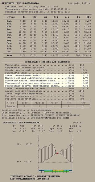
Bioclimatic Diagnosis: Temperate Oceanic Bioclimate,
Submediterranean
Variant
Figure 78
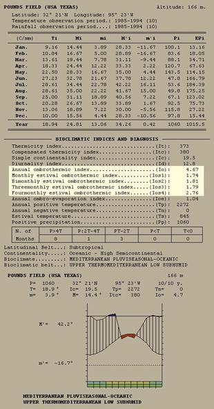
Bioclimatic Diagnosis: Mediterranean
Pluviseasonal Oceanic
Bioclimate,
Normal Variant
Figure 79
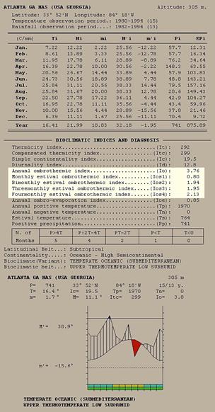
Bioclimatic Diagnosis: Temperate Oceanic Bioclimate,
Submediterranean Variant
10.- Itc and Ci CALCULATIONS
The Compensated Thermicity Index is used to
distinguish the Tropical, Mediterranean and Temperate Macrobioclimates, as well
as their Thermotypes. For its calculation it is necessary to take into account
the Latitude and the Continentality, since it is necessary to apply a
progressive correction factor, fi, according to the excess of cold or or heat due to
the Continentality / Oceanicity of the meteorological station under study. To
facilitate Itc calculation and knowledge, we will explain here, in
detail, the procedure to be used.
In Chapter 3 we
saw that the Compensated Thermicity Index is:
Itc
= It + Ci = (T + M + m) 10 + Ci
Expression
convertible into:
Itc
≈ (T + 2 Tmin) 10 + Ci
The first part
of the expression offers no calculation difficulties. But, as the compensation
value, Ci, varies according to Latitude and Continentality, in
Figure 80, we have collected, the Latitude and Continentality intervals, as
well as the progressive correction factor, fi, to be applied at each of their intervals, and,
finally, we have collected the calculations of Ci. The Continentality progressive correction factor - fi - reaches values between (-10) and (+30).
Figure 80. - Calculation of the compensation
values, Ci, to obtain the Compensated Thermicity Index - Itc -, according to
the Latitude and thresholds of Continentality, according to Rivas-Martínez.
|
Latitude |
-lc- Thresholds of Continentality |
|
|
Ci
Calculations |
|
Up to 23º N and S |
--- --- |
|
|
--- --- --- --- --- |
|
|
Ic≤8 |
|
|
C0=f0
(8 - Ic) |
|
|
fi = 0 |
Ci = 0 |
--- --- --- --- --- |
|
|
17<Ic≤
21 |
f1
= 5 |
Ci =Cl; |
C1=f1
(Ic - 17) |
|
|
21< Ic≤
28 |
f2
= 15 |
Ci = Cl
+ C2 |
C1=f1
(21 - 17) =20; C2=f2
(Ic - 21) |
|
|
28 < Ic ≤
46 |
f3
= 25 |
Ci =Cl
+ C2 + C3 |
C1=20;
C2=f2
(28 - 21) = 105; C3=f3
(Ic - 28) |
|
|
|
f4
= 30 |
Ci =Cl
+ C2 +C3 +
C4; |
C1=20;
C2=105;
C3=f3
(46 - 28) =450; C4=f4
(Ic - 46) |
In figures 81-87, we can see some case studies, with specific
meteorological stations, of the results for the Itc calculations, shown in
figure 80, as detailed below:
.) Between 23º
N and S, the compensation value, Ci, is equal to 0, because, at those latitudes, it is
not necessary to compensate neither the excess of cold nor the heat, due to low
or high Continentality. So in those latitudes: It = Itc (See figure 81, Ghanzi, Botswana).
.) At more than
23º N and S,
A) in the strongly
hyperoceanic areas (Ic ≤ 8), the compensation value, C0, is calculated by
multiplying by f0 = (-10) the difference between 8.0 and the Ic of the locality: C0 = (-10)
x (8.0 - Ic). (See Figure 82, Ushuaia, Argentina).
B) in low Continental
areas (8<Ic≤17), the value of Ci is considered equal to 0, so, in
these cases: It = Itc (See figure 83, Torgilsbu, Greenland-DNK).
C) in intermediate
Continental areas (17<Ic≤ 21), the compensation value, C1, is
calculated by multiplying by fi (f1 = 5)
the difference between the Ic of the locality and the value 17: C1=f1
(Ic – 17). (See Figure 84, Pingwu, China).
D) in the high
Continental areas (21<Ic≤ 28), the compensation value Ci is calculated
by a sum whose partial values Ci = C1 + C2, are as follows: C1=f1 (21 - 17)
=20; y C2=f2 (Ic - 21). See figure 85, Teheran-Doshant, Iran).
E) in very high
Continental areas (28 <Ic≤ 46), the compensation value Ci is
calculated by a sum whose partial values Ci = Cl + C2 + C3, are as follows:
C1=f1 (21 - 17) =20; C2=f2 (28 - 21) =105; y C3 = f3 (Ic - 28). (See Figure 86,
Lamaiin Huryee, Mongolia).
F) in extremely high
Continental areas (46<Ic≤ 65), the compensation value Ci is calculated
by a sum whose partial values Ci
= Cl + C2 + C3 + C4, are
as follows: C1=f1 (21 - 17) =20; C2=f2 (28 - 21) =105; C3 = f3 (46 - 28) = 450;
y C4 = f4 (Ic - 46). (See figure
87, Vakjanka, Russia).
Figure 81
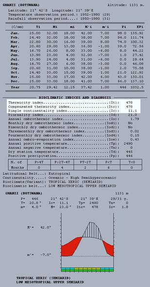
Bioclimatic
Diagnosis: Tropical Xeric
Bioclimate,
Normal
Variant
Figure 82
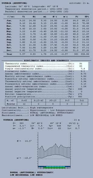
Bioclimatic Diagnosis: Boreal Hyperoceanic Bioclimate,
Normal
Variant
Figure 83
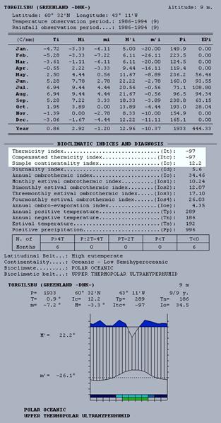
Bioclimatic Diagnosis: Polar Oceanic Bioclimate,
Normal
Variant
Figure 84
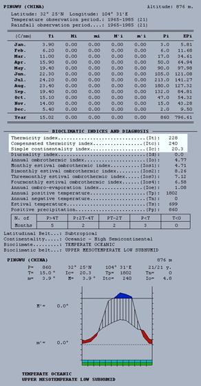
Bioclimatic Diagnosis: Temperate Oceanic Bioclimate,
Normal
Variant
Figure 85
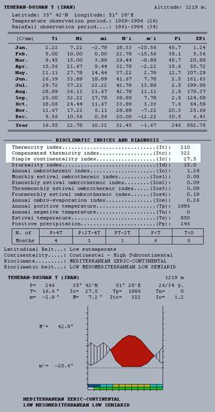
Bioclimatic
Diagnosis: Mediterranean Xeric
Continental Bioclimate, Normal Variant
Figure 86
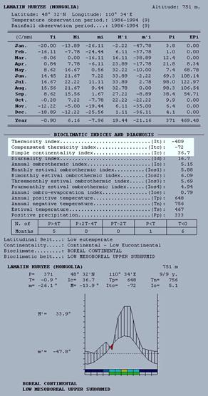
Bioclimatic
Diagnosis: Boreal Continental
Bioclimate,
Normal
Variant
Figure 87
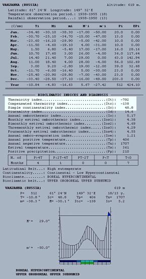
Bioclimatic Diagnosis: Boreal Hypercontinental Bioclimate,
Normal Variant
11.- PRACTICAL EXAMPLE of a meteorological station
complete bioclimatic characterization, with the use of the Synoptic Table.
In order to
facilitate the bioclimatic characterization of a meteorological station, we
will carry out, in detail, all the steps and calculations necessary for that
study, taking as a model the station of DZHEZKAZGÁN, located in the center of
Kazakstan. All the climatic data in this section are taken from Prof.
Rivas-Martínez's website: http://www.globalbioclimatics.org. (2008), but the
classification follows Rivas-Mart. & al., 2011.
We will do the
practical example according to the following scheme:
11.1.- Climatic data of
departure
11.2.- Bioclimatic
diagnosis of a weather station
11.2.a.- Location of the
weather station: Latitude, longitude and altitude
11.2.b.- Calculation of
the necessary values and indexes.
Three THERMAL INDEXES:
Ic Continentality / Oceanicity Index
Tp Positive Annual Temperature
Itc Compensated Thermicity Index
One OMBRIC (Rainfall)
INDEX
Pp Annual positive
precipitation
Four OMBROTHERMIC INDEXES
Io Annual Ombrothermic Index, Io = (Pp/Tp)10.
Ios2
Ombrothermic Index of the hottest bimester of the summer trimester
Iosc3 (= Ios3), Compensable Ombrothermic Index of the summer trimester,
necessary to evaluate the summer aridity
Iosc4 (= Ios4), Compensable Summer Ombrothermic Index for the four-month
period resulting from adding, to the summer trimester, the month immediately
preceding. This index is also used to assess summer aridity
11.2.c.- Recognition of
the bioclimatic units of the station, using the General Synoptic Table.
MACROBIOCLIMATE
BIOCLIMATE AND BIOCLIMATIC VARIANT
. BIOCLIMATE
. BIOCLIMATIC VARIANT
BIOCLIMATIC BELT: Thermotype and Ombrotype
11.2.d.- Expression of
the complete bioclimatic diagnosis -Isobioclimate-.
11.3.- Synthesis and
graphic expression of bioclimatic study: Bioclimograph
11.1.- Climatic data of departure
Figure 88
collects the information provided by a weather station, in this case, DZHEZKAZGAN,
Kazakhstan. It contains: a) latitude, longitude and altitude geographic data;
b), chronological data: temperatures and precipitation observation periods; And
c), climatic data: for the considered periods, the average monthly values of Ti (monthly average temperature), Mi (average of the maximums of each month), mi (average of the minimum of each month), M'i (average monthly temperature of absolute maximums), m'i (average monthly temperature of the absolute
minimums), and of Pi (mean of the monthly precipitations). Of all these data, those columns
that we need for our study, and that we are going to use are: Ti, Mi, mi, and Pi.
Figure 88.- Necessary data for the bioclimatic
study of a meteorological station: DZHEZKAZGAN
|
DZHEZKAZGAN, Kazakhstan |
||||||
|
Latitude: 47º 48'N Longitude: 067º 43'E Altitude: 345m |
||||||
|
Temperature observation period: 1968 -1994 (27) |
||||||
|
Rainfall observation period . . . . : 1984 -1994 (11) |
||||||
|
|
|
Mi |
|
|
|
|
|
Jan |
-16,1 |
-11,1 |
- 21,0 |
7,8 |
-50,0 |
14,5 |
|
|
|
- 9,4 |
|
|
|
|
|
Mar |
-7,2 |
-1,7 |
-12,8 |
25,0 |
-38,9 |
25,9 |
|
|
6,4 |
13,3 |
-0,6 |
|
|
|
|
May |
15,0 |
23,3 |
6,7 |
67,8 |
- 8,9 |
14,0 |
|
Jun |
20,8 |
29,4 |
12,2 |
41,1 |
-1,1 |
22,6 |
|
|
|
31,7 |
|
|
|
|
|
Aug |
|
29,4 |
12,2 |
41,1 |
0,0 |
8,1 |
|
Sep |
13,9 |
22,8 |
5,0 |
37,2 |
-10,0 |
8,4 |
|
|
|
12,2 |
|
|
|
|
|
Nov |
|
0,6 |
-10,0 |
18,9 |
- 38,9 |
9,7 |
|
Dec |
-13,1 |
-7,8 |
-18,3 |
6,1 |
- 41,1 |
13,2 |
|
Year |
--- |
--- |
--- |
--- |
--- |
--- |
Note:
The data source can already give us the annual values, but if not, we
ourshelves calculate them: the annual temperature values are the arithmetic
mean of the corresponding monthly mean values; with respect to annual rainfall,
simply add up all the monthly values: Figure 89.
Figure 89.- Mean annual data of temperatures and
average total rainfall calculated for the DZHEZKAZGAN Meteorological Station:
|
DZHEZKAZGAN, Kazakhstan |
||||||
|
Latitude: 47º 48'N Longitude: 067º 43'E Altitude: 345m |
||||||
|
Temperature observation period: 1968 -1994 (27) |
||||||
|
Rainfall observation period . . . . : 1984 -1994 (11) |
||||||
|
|
|
Mi |
|
|
|
|
|
Jan |
-16,1 |
-11,1 |
- 21,0 |
7,8 |
-50,0 |
14,5 |
|
|
|
- 9,4 |
|
|
|
|
|
Mar |
-7,2 |
-1,7 |
-12,8 |
25,0 |
-38,9 |
25,9 |
|
|
6,4 |
13,3 |
-0,6 |
|
|
|
|
May |
15,0 |
23,3 |
6,7 |
67,8 |
- 8,9 |
14,0 |
|
Jun |
20,8 |
29,4 |
12,2 |
41,1 |
-1,1 |
22,6 |
|
|
|
31,7 |
|
|
|
|
|
Aug |
|
29,4 |
12,2 |
41,1 |
0,0 |
8,1 |
|
Sep |
13,9 |
22,8 |
5,0 |
37,2 |
-10,0 |
8,4 |
|
|
|
12,2 |
|
|
|
|
|
Nov |
|
0,6 |
-10,0 |
18,9 |
- 38,9 |
9,7 |
|
Dec |
-13,1 |
-7,8 |
-18,3 |
6,1 |
- 41,1 |
13,2 |
|
Year |
T = 4,1 |
--- |
--- |
--- |
--- |
P = 175,8 |
11.2.- Bioclimatic diagnosis of a weather station
From the
climatic data emitted by the meteorological station, collected and synthesized
in Figures 88 and 89, four are the necessary steps to perform the bioclimatic
diagnosis of the locality: a, take into account the geographic location - latitude, longitude and
altitude - of the weather station; b,
calculation of the necessary values and indexes; c, recognition of the bioclimatic units of the station, with the
help of the Synoptic General Table; and d,
complete formulation of Isobioclimate.
11.2.a.- Location of the weather station: Latitude,
longitude and altitude
When starting
the bioclimatic study of a station / locality, since that geographical position
conditions the monthly distribution of the seasons spring, summer, autumn and
winter. The table, as it is usually written, always starts in January. If the
station was located inthe Southern Hemisphere, it is convenient to draw, in the
data table, a horizontal line of separation between May and June, because in
that hemisphere the winter begins in June.
11.2.b.- Calculation of the necessary values and
indexes.
For more ease, we are going to first compute three Thermal Indices,
then one Index of rainfall, to end up with four Ombrothermal Indexes.
Three THERMAL INDEXES:
Continentality / Oceanicity Index: Annual thermal amplitude - Ic - The Index expresses the
difference, in degrees centigrade, between the highest and lowest monthly
average temperatures of the year:
Ic = Tmax – Tmin
To calculate it at our station - Figure 90- we go to the Ti column, of
average monthly temperatures, and we look for the months with the highest and
lowest values, which are those of July and January.
Figure 90.- The data for the calculation of the
Continental Index are marked
|
DZHEZKAZGAN,
Kazakhstan |
||||||
|
|
||||||
|
Temperature
observation period: 1968 -1994 (27) |
||||||
|
|
||||||
|
|
|
Mi |
|
|
|
|
|
Jan |
-16,1 |
-11,1 |
- 21,0 |
7,8 |
-50,0 |
14,5 |
|
|
|
- 9,4 |
|
|
|
|
|
Mar |
-7,2 |
-1,7 |
-12,8 |
25,0 |
-38,9 |
25,9 |
|
|
6,4
|
13,3 |
-0,6
|
|
|
|
|
May |
15,0 |
23,3 |
6,7 |
67,8 |
- 8,9 |
14,0 |
|
Jun |
20,8 |
29,4 |
12,2 |
41,1 |
-1,1 |
22,6 |
|
|
|
31,7 |
|
|
|
|
|
Aug |
|
29,4 |
12,2 |
41,1 |
0,0 |
8,1 |
|
Sep |
13,9 |
22,8 |
5,0 |
37,2 |
-10,0 |
8,4 |
|
|
|
12,2 |
|
|
|
|
|
Nov |
|
0,6 |
-10,0 |
18,9 |
- 38,9 |
9,7 |
|
Dec |
-13,1 |
-7,8 |
-18,3 |
6,1 |
- 41,1 |
13,2 |
|
Year |
T = 4,1 |
--- |
--- |
--- |
--- |
P =
175,8 |
Ic=+23,1 – (-16,1) = 39,2
Positive Annual Temperature - Tp -: It is the sum, expressed in tenths of degree
centigrade, of the average monthly temperatures of those months that exceed
0ºC: Ti > 0ºC. Tp = ∑
Ti (Ti > 0) x 10, being i: 1 = January, ..., 12 = December.
Figure 91.- The data for the calculation of the
Annual Positive Temperature in the station of
DZHEZKAZGAN are marked
|
DZHEZKAZGAN,
Kazakhstan |
||||||
|
|
||||||
|
Temperature
observation period: 1968 -1994 (27) |
||||||
|
|
||||||
|
|
|
Mi |
|
|
|
|
|
Jan |
-16,1 |
-11,1 |
- 21,0 |
7,8 |
-50,0 |
14,5 |
|
|
|
- 9,4 |
|
|
|
|
|
Mar |
-7,2 |
-1,7 |
-12,8 |
25,0 |
-38,9 |
25,9 |
|
|
6,4
|
13,3 |
-0,6
|
|
|
|
|
May |
15,0 |
23,3 |
6,7 |
67,8 |
- 8,9 |
14,0 |
|
Jun |
20,8 |
29,4 |
12,2 |
41,1 |
-1,1 |
22,6 |
|
|
|
31,7 |
|
|
|
|
|
Aug |
|
29,4 |
12,2 |
41,1 |
0,0 |
8,1 |
|
Sep |
13,9 |
22,8 |
5,0 |
37,2 |
-10,0 |
8,4 |
|
|
|
12,2 |
|
|
|
|
|
Nov |
|
0,6 |
-10,0 |
18,9 |
- 38,9 |
9,7 |
|
Dec |
-13,1 |
-7,8 |
-18,3 |
6,1 |
- 41,1 |
13,2 |
|
Year |
T = 4,1 |
--- |
--- |
--- |
--- |
P =
175,8 |
In our station -
Figure 91- we have to add Ti from April to October inclusive and multiply the result by 10, to
express it in tenths of a degree, so our
Tp = (6,4 + 15,0 + 20,8 +
23,1 + 20,8 + 13,9 + 5,0) 10 = 1050
Compensated Thermicity Index -Itc-
It is the sum,
in tenths of a degree, of T (annual mean temperature), M (average temperature of the maximum of the coldest
month, ie of the month with the lowest Ti) and m (average temperature of the minimums of the coldest
month, that is the month with the lowest Ti), plus a compensation value, Ci:
Itc = (T + M + m)10 + Ci
The compensation
value Ci must be applied to correct the excess of
"temperance" or "cold" that occurs when the Continentality
Index is extremely low (Ic ≤ 8), or high (Ic>18), compared to cases where the lc has mean values, between 8-18: thus, the values
obtained with the ltc are comparable.
Performing the calculations:
1st
stage: Calculation of
the first part of the formula: (T + M + m) 1O. At our DZHEZKAZGAN station, the coldest month-the one
with the lowest monthly average temperature-is January, Figure 92, so that
(T + M + m) 1O = [(+4,1) + (-11,1) +
(-21)]10 = (-28,1x10) = - 281
Figure 92.- The data for the calculation of the
Compensated Termicity Index, in the DZHEZKAZGAN station, are marked
|
DZHEZKAZGAN,
Kazakhstan |
||||||
|
|
||||||
|
Temperature
observation period: 1968 -1994 (27) |
||||||
|
|
||||||
|
|
|
Mi |
|
|
|
|
|
Jan |
-16,1 |
-11,1 |
- 21,0 |
7,8 |
-50,0 |
14,5 |
|
|
|
- 9,4 |
|
|
|
|
|
Mar |
-7,2 |
-1,7 |
-12,8 |
25,0 |
-38,9 |
25,9 |
|
|
6,4
|
13,3 |
-0,6
|
|
|
|
|
May |
15,0 |
23,3 |
6,7 |
67,8 |
- 8,9 |
14,0 |
|
Jun |
20,8 |
29,4 |
12,2 |
41,1 |
-1,1 |
22,6 |
|
|
|
31,7 |
|
|
|
|
|
Aug |
|
29,4 |
12,2 |
41,1 |
0,0 |
8,1 |
|
Sep |
13,9 |
22,8 |
5,0 |
37,2 |
-10,0 |
8,4 |
|
|
|
12,2 |
|
|
|
|
|
Nov |
|
0,6 |
-10,0 |
18,9 |
- 38,9 |
9,7 |
|
Dec |
-13,1 |
-7,8 |
-18,3 |
6,1 |
- 41,1 |
13,2 |
|
Year |
T = 4,1 |
--- |
--- |
--- |
--- |
P =
175,8 |
2nd
stage: Ci
calculation. As we saw in Chapter 10, Ci value is calculated according to the
latitude and to the different thresholds of Continentality, established by
Rivas-Martínez (see Figure 93). Latitude thresholds: up to 23º N and S, and
greater than 23º N and S. Continentality thresholds: from 0 to 8, up to 17, up
to 21, up to 28, up to 46 and up to 65. The last column gives the highest
values of Ci that can be reached at each Continental threshold.
For our weather station of DZHEZKAZGAN, we have to
take into account the Index of Continentality previously calculated: lc = 39.2.
That is why we have to apply the content of the threshold line 28 <Ic≤46.
(Figure 93), in which our Ci= C1 + C2 + C3, being C1=20; C2=105; and C3=f3 (lc
- 28) = 25(39,2-28) =25 x 11,2 = 280. With it Ci =C1 + C2 + C3 = 15+ 105 + 280
= +405. So:
Ci = +405
Figure 93. Calculation of compensation values Ci
needed for the Compensated Thermicity Index - Itc, according to the thresholds
of Continentality of Rivas Martínez. The calculation of the Compensated
Thermicity Index for the DZHEZKAZGAN station has been indicated.
|
Latitude |
-lc-
Thresholds of Continen-tality |
|
|
Ci
Calculations |
Valores Extremos de
Ci |
|
Up to 23º N and S |
--- --- |
|
|
--- --- --- --- --- |
Ci = 0 |
|
|
Ic≤8 |
|
|
C0=f0
(8 - Ic) |
C0 = - 80 |
|
|
fi = 0 |
Ci = 0 |
--- --- --- --- --- |
Ci = 0 |
|
|
17<Ic≤
21 |
f1
= 5 |
Ci i=Cl; |
C1=f1
(Ic - 17) |
C1 = + 20 |
|
|
21< Ic≤
28 |
f2
= 15 |
Ci = Cl
+ C2 |
C1=f1
(21 - 17) =20; C2=f2
(Ic - 21) |
C2 = + 105 |
|
|
28 < Ic ≤
46 |
f3
= 25 |
Ci =Cl
+ C2 + C3 |
C1=20;
C2=f2
(28 - 21) = 105; C3=f3
(Ic - 28) |
C3 = + 450 |
|
|
|
f4
= 30 |
Ci =Cl
+ C2 +C3 +
C4; |
C1=20;
C2=105;
C3=f3
(46 - 28) =450; C4=f4
(Ic - 46) |
C4 = +570 |
3rd stage: Calculation of Itc. Finally, we only need,
in this third stage, to make the final calculation:
Itc = (T + M + m)10 + Ci = -281 + 405 = 124
Note: Itc can be calculated, even if the averages of the monthly
maximums and minimums are not available, because (M + m) is approximately 2Tmin
(Tmin: Monthly average temperature of the coldest month of the year):
Itc ≈ (T + 2Tmin)10 +
Ci = [4,1 +2(-16,1)]10 + 405 = -281 + 405 = 124
One RAINFALL INDEX
Annual Positive Precipitation –Pp- is the sum of Pi of all months of the year, whose Ti is greater than 0ºC. Pp=∑Pi (Ti>0), being i: 1 = January, ..., 12 = December.
In our case -
Figure 94 - we must add the monthly precipitations from April to October: Pp = 97. (rounding off 96.5).
Pp = 6,6 + 14,0 + 22,6 +
19,8 + 8,1 + 8,4 + 17,0 = 97
Figure 94.- The data for the calculation of the
Positive Precipitation in the meteorological station of DZHEZKAZGAN are marked.
|
DZHEZKAZGAN,
Kazakhstan |
||||||
|
|
||||||
|
Temperature
observation period: 1968 -1994 (27) |
||||||
|
|
||||||
|
|
|
Mi |
|
|
|
|
|
Jan |
-16,1 |
-11,1 |
- 21,0 |
7,8 |
-50,0 |
14,5 |
|
|
|
- 9,4 |
|
|
|
|
|
Mar |
-7,2 |
-1,7 |
-12,8 |
25,0 |
-38,9 |
25,9 |
|
|
6,4
|
13,3 |
-0,6
|
|
|
|
|
May |
15,0 |
23,3 |
6,7 |
67,8 |
- 8,9 |
14,0 |
|
Jun |
20,8 |
29,4 |
12,2 |
41,1 |
-1,1 |
22,6 |
|
|
|
31,7 |
|
|
|
|
|
Aug |
|
29,4 |
12,2 |
41,1 |
0,0 |
8,1 |
|
Sep |
13,9 |
22,8 |
5,0 |
37,2 |
-10,0 |
8,4 |
|
|
|
12,2 |
|
|
|
|
|
Nov |
|
0,6 |
-10,0 |
18,9 |
- 38,9 |
9,7 |
|
Dec |
-13,1 |
-7,8 |
-18,3 |
6,1 |
- 41,1 |
13,2 |
|
Year |
T = 4,1 |
--- |
--- |
--- |
--- |
P =
175,8 |
Four OMBROTHERMIC
INDEXES
Their values
areten times the quotient between Positive Precipitation and Positive
Temperature of the considered period, Io
= (Pp / Tp) 10. In addition to the Io, Annual Ombrothermal Index, it is
necessary to calculate the Ombrothermal Indexes for the summer period -
Jun-Jul-Aug, in the Northern Hemisphere; Dec-Jan-Feb, in the Southern
Hemisphere:
Io Annual Ombrothermic Index
Ios2 Ombrothermic Index of the hottest bimester
of the summer trimester (Tr3)
Iosc3 (= Ios3) Compensable Ombrothermic Index of the
summer trimester (Tr3)
Iosc4 (= Ios4) Compensable Summer
Ombrothermic Index for the four-month period resulting from adding, to the
summer trimester (Tr3), the month immediately preceding.
We calculate
each of them: Figure 95.
Figure 95.- The data for the calculation of the
Summer Ombrothermal Indexes are marked in the meteorological station of
DZHEZKAZGAN.
|
DZHEZKAZGAN, Kazakhstan |
||||||
|
|
||||||
|
Temperature observation period: 1968 -1994 (27) |
||||||
|
|
||||||
|
|
|
Mi |
|
|
|
|
|
Jan |
-16,1 |
-11,1 |
- 21,0 |
7,8 |
-50,0 |
14,5 |
|
|
|
- 9,4 |
|
|
|
|
|
Mar |
-7,2 |
-1,7 |
-12,8 |
25,0 |
-38,9 |
25,9 |
|
|
6,4 |
13,3 |
-0,6 |
|
|
|
|
May |
15,0 |
23,3 |
6,7 |
67,8 |
- 8,9 |
14,0 |
|
Jun |
20,8 |
29,4 |
12,2 |
41,1 |
-1,1 |
22,6 |
|
|
|
31,7 |
|
|
|
|
|
Aug |
|
29,4 |
12,2 |
41,1 |
0,0 |
8,1 |
|
Sep |
13,9 |
22,8 |
5,0 |
37,2 |
-10,0 |
8,4 |
|
|
|
12,2 |
|
|
|
|
|
Nov |
|
0,6 |
-10,0 |
18,9 |
- 38,9 |
9,7 |
|
Dec |
-13,1 |
-7,8 |
-18,3 |
6,1 |
- 41,1 |
13,2 |
|
Year |
T = 4,1 |
--- |
--- |
--- |
--- |
P = 175,8 |
Annual Ombrothermic Index, Io = (Pp/Tp)10.
With the values
of Pp and Tp, calculated above, Pp = 97; Tp = 1050:
Io = (Pp/Tp)10 = (97
/ 1050)10 = 0,92
Ombrothermic Index of the hottest bimester of the
summer trimester (Tr3):
Ios2: = (Pp2/Tp2) 10
As
Pp2 = 19,8+8,1=27,9; and Tp2 = (23,1+20,8) x 10 =439:
Ios2: = (Pp2/Tp2) 10 = (27,9 /
439)10 = 0,64
Compensable Ombrothermic Index of the summer trimester (Tr3): Iosc3 = (Pp3/Tp3) 10:
As
Pp3 = 19,8+8,1+22,6=50,5; and Tp3 = (20,8+23,1+20,8) 10 =647:
Iosc3 = (50,5 / 647) 10 = 0,78
Compensable Summer Ombrothermic Index for the
four-month period
resulting from adding, to the summer trimester (Tr3), the month immediately preceding.
Iosc4
= (Pp4/Tp4) 10:
As
Pp4=19,8+8,1+22,6+14=64,5; and Tp4= (20,8+23,1+20,8+15) x 10 =797:
Iosc4 = (64,5 / 797) 10 = 0,81
11.2.c.- Recognition of the bioclimatic units of the
station, using the General Synoptic Table.
Once the
latitude, longitude and height data are recognized, and the calculations of the
indices of our DZHEZKAZGAN station are carried out, we will identify its
Bioclimatology having in view the General Synoptic Table of the Bioclimatic
Classification of the Earth (figure 7). We have to find out what
Macrobioclimate, what Bioclimate and Bioclimatic Variant, and what Bioclimatic
Belt correspond to it, to finally define the Isobioclimate of DZHEZKAZGAN.
MACROBIOCLIMATE
In the
Macrobioclimates column of the Synoptic General Table, the first thing we
encounter is the call: (1). And is
that to identify the Macrobioclimate, in addition to latitude, thermal
thresholds T, M, m, Itc and Tp are used, all of them highly conditioned by the altitude of the
meteorological station. As the Synoptic Table gives the thresholds of those
indices referred to 200m, if our station exceeds that altitude, we must add a
certain amount for every 100m that exceeds 200m. The amount to be added to each
index is indicated in the call (1) of the Synoptic Table, column of Macrobioclimates,
column shown in figure 96.
Figure 96. Recognition of the Macrobioclimate at
the DZHEZKAZGAN station. First column of the Synoptic Table
|
M a c r o b i o c l i m a t e s(1) |
|
Name, Acronym and Differential Characters |
|
Tropical Tr Warm zone: equatorial, eutropical and subtropical
(0º-35º N & S). In subtropical (23º - 35º N & S) at < 200 m, at
least two values: T ≥ 25º, m ≥ 10º, Itc ≥ 580; or, if Pss
> Psw, or Pcm2 < Pcm1 > Pcm3, at least two values: T ≥ 21º, M ≥
18º, Itc ≥ 470. In Eurasia, from 25º to 35º N, height ≥ 2000 m:
it is not tropical. |
|
Medit Subtropical
warm zone (23º-35º N & S) and eutemperate
temperate zone (35º-52º N & S), with
summer aridity at least bimonthly after the summer solstice: Ios2 ≤ 2, Iosc4
≤ 2. In Subtropical, at least two of the three thermal values: T < 25º,
m < 10º, Itc < 580.
|
|
Temperate Te Subtropical
warm zone (23º-35º N & S) and temperate
zone (35º-66º N & 35º-54º S). Without
summer aridity: Ios2>2, Iosc4>2. A <200 m, Tp≥380.
Besides: a), 23º-35º N & S, at <200m, at least two values: T<21º,
M<18º, Itc<470; or b), In contrast to Boreal, at <200m: if Ic≤11:
T>6º, Tmax>10º and Tps>320; if 11<Ic≤21: Tp>720 and T>5.3º; if 21<Ic≤28: Tp>740 and T>4.8º; if 28<Ic≤46:
Tp>800 and T>3.8º; and if 46<Ic: Tp>800 and T>0º.
|
|
Boreal Bo Temperate and cold zones (42º-72º N, 49º-56º S). Without summer aridity:
Ios2>2, Iosc4>2. A <200 m, Tp≥380. If Ic≤11: T≤6º, Tmax≤10º, 380≤Tp≤720 and Tps≤320; if 11<Ic≤21: 380≤Tp≤720 and T≤5.3º; if 21<Ic≤28: 380≤Tp≤740 and T≤4.8º; if 28<Ic≤46:
380≤Tp≤800 and T≤3,8º; and if 46<Ic: 380≤Tp≤800 and T≤0º. |
|
Polar Po Temperate
and cold zones (51º-90º N & S). Altitude < 100m: Tp < 380.
(Rivas-Mart. et al., 2011)
(Modificado M.L. López
y M.S. López, 26 diciembre 2016) |
|
(1) Between 23º - 48º N and 23º - 51º S, if the locality is to 200 m,
or more, of altitude, the thermal values must theoretically be calculated at
such a height increasing T by 0.6º; M and m, by 0.5 °; and Itc by 13 units,
per every 100 m that exceeds that altitude. At more than 48 ° N or 51 ° S, it
is necessary to calculate the theoretical values of the average annual
temperature, the average of the maximums of the coldest month, and the annual
positive temperature, increasing T by 0.4 °, M by 0.5 ° and Tp by 12 units,
for every 100 m exceeding said altitude. |
DZHEZKAZGAN is
located at 345m s.n.m., so that exceeds in 145m the 200m of reference. In
Figure 97, the real values of de T, M, Itc and Tp are collected, as well as the theoretical values that result from
theoretically positioning the station at 200m.
Figure 97.- Calculation of the theoretical values
of the station of DZHEZKAZGAN, at 200m.
|
Increase per every 100m |
DZHEZKAZGAN, at 345m |
DZHEZKAZGAN, at 200m |
|
T + 0,6º/100m |
T = 4,1 |
T + 0,6º = 4,7 |
|
M + 0,5º/100m |
M = -11,1 |
M + 0,5º = -10,6 |
|
Itc + 13/100m |
Itc = 119 |
Itc + 13 = 132 |
|
Tp + 55/100m |
1050 |
Tp + 55 = 1105 |
Once we have met
the call (1), we can begin to analyze the Macrobioclimate of our meteostation.
We look at the Macrobioclimates column of Figure 96: The first character
mentioned is latitude. Latitude of Dzhezkazgán, 47º48'N. We have shaded the
latitudes of the three possible Macrobioclimates, which could fit Dzhezkazgan:
Mediterranean, Temperate and Boreal.
To distinguish
now between these three Macrobioclimates, we analyze the following character:
summer aridity, that is, if Ios2 is less than or equal to 2, or greater than 2. As our Ios2 = 0.64, it seems that our meteostation is
Mediterranean: but before giving it as definitive, we have to check for a
possible compensation by the moisture retained in the soil, due to rainfall in
the month, or in the previous two months, by using the values of Iosc3, Iosc4.
To analyze the
possible compensation, we look at figure 72. It is clear that, in order to
assess the possible compensation of the summer aridity of an Ios2≤2, the annual Io must be equal to or greater than 2. In
our case of DZHEZKAZGAN, its Io = 0.92, less than 2, does not even allow us to start the query of
possible compensation, so our station has, definitely, summer aridity and is,
therefore, Mediterranean.
From the
Macrobioclimates column, figure 96, it follows that, of the three possible
Macrobioclimates by latitude, only the Mediterranean Macrobioclimate has summer
aridity, which leads us to conclude that:
Dzhezkazgán
has a Mediterranean Macrobioclimate
BIOCLIMATE AND BIOCLIMATIC VARIANT
Once we know the
Macrobioclimate of our station as Mediterranean, we proceed as follows for the
identification of the Bioclimate / Bioclimatic Variant:
Figure 98. Differential characteristics of the
Mediterranean Bioclimates, according to the Bioclimatic Synopsis of the Earth.
|
Mediterranean Bioclimates |
Bioclimatic intervals |
Acronyms |
|
|
Io |
Ic |
||
|
Me.
Pluviseasonal Oceanic |
2.0≤Io |
≤ 21 |
Mepo |
|
Me.
Pluviseasonal Continental |
2.0≤Io |
> 21 |
Mepc |
|
Me.
Xeric Oceanic |
1.0≤Io<2.0 |
≤ 21 |
Mexo |
|
Me.
Xeric Continental |
1.0≤Io<2.0 |
> 21 |
Mexc |
|
Me. Desertic Oceanic |
0.2≤Io<1.0 |
≤ 21 |
Medo |
|
Me. Desertic Continental |
0.2≤Io<1.0 |
> 21 |
Medc |
|
Me.
Hyperdesertic Oceanic |
Io<0.2 |
≤ 21 |
Meho |
|
Me.
Hyperdesertic Continental |
Io<0.2 |
> 21 |
Mehc |
For the BIOCLIMATE,
we go to the second column-second row of the General Synopsis (Figure 7), which
is reproduced in Figure 98. Analyzing the bioclimatic intervals that define each
of the Mediterranean Bioclimates, we see that the Ombrothermal Index of our
station, Io = 0.92, is in between 0.2 and 1.0, making it a Mediterranean
Desertic Bioclimate. As there are two Bioclimates with that denomination, we
now look at the Station's Continentality Index, which is Ic = 39.2,
continental. So that:
Dzhezkazgán has a
Mediterranean Desertic Continental Bioclimate
Regarding the BIOCLIMATIC
VARIANT, in the General Synoptic Table, (figure 7), we found that, in that
Bioclimate, only two variants - Steppe and Normal-, have been observed. We now
check if our meteostation meets the requirements of the Steppic Variant,
because otherwise, it would be the Normal Variant.
Figure 99.- The data to be used fot analyzing the
possible existence of a Steppic Variant in DZHEZKAZGAN, are marked.
|
DZHEZKAZGAN, Kazakhstan |
||||||
|
|
||||||
|
Temperature observation period: 1968 -1994 (27) |
||||||
|
|
||||||
|
|
|
Mi |
|
|
|
|
|
Jan |
-16,1 |
-11,1 |
- 21,0 |
7,8 |
-50,0 |
14,5 |
|
|
|
- 9,4 |
|
|
|
|
|
Mar |
-7,2 |
-1,7 |
-12,8 |
25,0 |
-38,9 |
25,9 |
|
|
6,4 |
13,3 |
-0,6 |
|
|
|
|
May |
15,0 |
23,3 |
6,7 |
67,8 |
- 8,9 |
14,0 |
|
Jun |
20,8 |
29,4 |
12,2 |
41,1 |
-1,1 |
22,6 |
|
|
|
31,7 |
|
|
|
|
|
Aug |
|
29,4 |
12,2 |
41,1 |
0,0 |
8,1 |
|
Sep |
13,9 |
22,8 |
5,0 |
37,2 |
-10,0 |
8,4 |
|
|
|
12,2 |
|
|
|
|
|
Nov |
|
0,6 |
-10,0 |
18,9 |
- 38,9 |
9,7 |
|
Dec |
-13,1 |
-7,8 |
-18,3 |
6,1 |
- 41,1 |
13,2 |
|
Year |
T = 4,1 |
--- |
--- |
--- |
--- |
P =175,8 |
The Steppic Variant implies: 1, a medium or high
Continentaity: Ic > 17;
2, an Ombrothermal Index between the lower hyperarid and the upper sub-humid: 6.0 ≥ Io > 0.2; 3, at least one summer month whith the
precipitation, in mm, less than three times its temperature, in degrees
centigrade: Psi < 3Ti;
-; and 4, the summer trimester positive precipitation needs to be higher than
the winter trimester positive precipitation: Pps>Ppw.
According to the results of our previous calculations,
in Dzhezkazgan: lc = 39.2; and
lo
= 0.92: we see
that it fulfills those two conditions. For the relation of the precipitation of
each summer month with its corresponding temperature, we take the data selected
in figure 99, and analyze them in figure 100.
Figure 100.- Calculations to check if the Psi
< 3Ti relation is fulfilled in the DZHEZKAZGAN station.
|
Mes |
Psi |
Ti |
Ti x 3 |
Relation Psi - 3Ti |
|
Jun |
22,6 |
20,8 |
62,4 |
22,6 < 62,4 |
|
Jul |
19,8 |
23,1 |
69.3 |
19,8 < 69.3 |
|
Aug |
8,1 |
20,8 |
62.4 |
8,l < 62.4 |
We find that not only one, but all the summer months
have Psi < 3Ti. That is, the station fulfills the third condition.
Let us see that the fourth condition is also fulfilled, that PpS>PpW. To check this fourth condition, we also take the
data from Figure 98, and analyze them in Figure 99, where we see how PpS>PpW: see figure 101.
Figure 101.- Calculations to check the relation
PpS>PpW, in the station of DZHEZKAZGAN
|
Summer Trimester Positive
Precipitation, Pps |
Winter Trimester Positive
Precipitation, Ppw |
Relation
Pps: Ppw |
||
|
Jun |
22,6 |
Dec |
0,0 |
|
|
Jul |
19,8 |
Jan |
0,0 |
|
|
Aug |
8,1 |
Feb |
0,0 |
|
|
Total |
50,5 |
Total |
0,0 |
Pps > Ppw |
As our station fulfills the four conditions of the
Steppic Variant, we can state that Dzhezkazgán has the following Bioclimate and
Variant:
Mediterranean Desertic
Continental, Steppic Variant
BIOCLIMATIC BELT -Thermotype and Ombrotype-
Bioclimatic
Belts are each one of the environments that follow each other in a latitudinal,
longitudinal or altitudinal cliserie. Each Bioclimatic Belt corresponds to
certain formations and plant communities: a vegetation belt. Each one of those
environments delimits values intervals of Itc, Tp -Termotypes-, and of Io -Ombrotypes-.
To determine the
Bioclimatic belt we have to go to the General Synopsis (figure 7) and observe
the columns corresponding to Bioclimatic Belts of the row Mediterranean
Macrobioclimate, columns that we have copied in Figures 102 and 103. In
Termotypes there is a call, clarified in the last lines of the table, which
warns us that, if the Continentality is high, Ic
≥ 21, or if the
Compensated Thermicity Index is low, Itc <120, the Thermotype is evaluated as a function of Tp.
Recall that Dzhezkazgán has lc = 39.2, ltc = 119,
Tp = 1050 and lo = 0.92. As our lc is high and, in addition, our ltc is low, we turn to the value of Tp =1050, between 900 and 1500, so our Thermotype is Supramediterranean. As for the
Ombrotype, our lo=0.92 falls
into the range 0.4 - 1.0, that is, the meteostation is Arid.
Thus, the
Bioclimatic Belt corresponding to Dzhezkazgán is:
Supramediterranean
Arid
Figure 102.- Bioclimatic Belts -Termotypes- of
the Mediterranean Macrobioclimate, extracted from the General Synopsis.
|
Bioclimatic
Belt |
Thermotype (2) |
Acronym |
|
|
Itc |
Tp (2) |
||
|
1 Inframediterranean |
450<ltc≤580 |
2400<Tp |
lme |
|
2 Termomediterranean |
350<ltc≤450 |
2100<Tp≤2400 |
Tme |
|
3 Mesomediterranean |
220<ltc≤350 |
1500<Tp≤2100 |
Mme |
|
4 Supramediterranean |
Itc ≤ 220 |
900<Tp≤1500 |
Sme |
|
5 Oromediterranean |
|
450<Tp≤900 |
Ome |
|
6 Crioromediterranean |
|
0<Tp≤450 |
Cme |
|
7 Gelid-mediterranean |
|
Tp=0 |
Gme |
|
(2) When Ic ≥ 21
(Continental) or when the values of Itc
<120, the Thermotype is calculated as a function of Tp, and the theoretical values of Tp at 200 are calculated by increasing 55 units per each 100m
that exceeds said altitude. |
|||
Figure 103.- Bioclimatic Belts -Ombrotypes- of
the Mediterranean Macrobioclimate, extracted from the General Synopsis
|
Bioclimatic
Belt |
Ombrotype
|
Acronym |
|
1 Ultrahyperarid |
Io < 0.2 |
Uha |
|
|
|
|
|
|
|
|
|
4 Semiarid |
1.0 ≤ Io < 2.0 |
Sar |
|
|
|
|
|
6 Subhumid |
3.6 ≤ Io < 6.0 |
Shu |
|
|
|
|
|
|
|
|
|
9 Ultrahyperhumid |
24.0 ≤ Io |
Uhh |
If we wanted to
express the Bioclimatic Belt as Termotypic and Ombrotypic Bioclimatic Horizons,
we would look at whether the values of Tp and Io are in the lower half, or in the upper half, of the thermal and ombric
intervals of the Bioclimatic Belt.
In our
meteostation of Dzhezkazgan, the Bioclimatic Horizons are:
Upper
Supra-Mediterranean, Upper Arid
11.2.d.- Expression of the complete bioclimatic
diagnosis -Isobioclimate-.
The
Isobioclimate, the basic unit of "Global Bioclimatics", expresses all
the climatic factors that operate in an area, and factors that explain the
presence in such area of a certain type of life. To name each Isobioclimate is
used a phrase that includes: Bioclimate / Bioclimatic Variant, together with a
Bioclimatic Belt - Thermotype + Ombrotype-.
With all the
known data we can, therefore, express the Isobioclimate
of our station of Dzhezkazgán, like
this:
Mediterranean Desertic
Continental, Steppic Variant, Supramediterranean, Arid
In addition to
words, the Isobioclimate can also be expressed by acronyms, recorded in the
General Synoptic Table:
Medc Stp Sme Ari
If more detail is needed, for a finer approximation to the
distribution of vegetation, We
have discussed above that the Bioclimatic Belt can be expressed as Bioclimatic
Horizons, the upper half or the lower half of the Thermotype and the Ombrotype.
It is how Rivas-Martínez names the Isobioclimate in his web, and as it also
appears named in Rivas-Mart. et al. 2011:
Mediterranean
Desertic Continental, Steppic Variant, Upper Supramediterranean, Upper Arid,
which, if we
express it in acronyms, results:
Medc Stp USme Uari
11.3.- Synthesis and graphic expression of bioclimatic
study: Bioclimograph
Everything done
in this practical example for the bioclimatic characterization of a
meteorological station appears in figure 104 (page 140), which is how the
climatic stations studied in the web "globalbioclimatics.org", of
Rivas-Mart. & Rivas-Sáenz (1996-2017), appear.
Figure 104 has
three parts: The first one contains the climatic data emitted by the station in
question, as well as its name, its geographic location and its periods of observation.
The second part shows the results of the necessary calculations to know the
Bioclimatic Indexes, as well as the resulting Bioclimatic Diagnosis. And in the
third part, the graphical representation of the Isobioclimate is given, that is
to say, its Bioclimogram (Ombro-Thermoclimograph or Ombro-Thermoclimogram).
Figure
104.- Bioclimatic study of Dzhezkazgán
|
|
|
|
|
|
|
|
|
|
Mediterranean Desertic Continental Bioclimate, Steppic Variant |
|

12.- BIOCLIMATIC CARTOGRAPHY
Knowing the
bioclimatic diagnosis of the meteorological stations of a continent, a region,
or a nation, etc., It is possible to draw the boundaries of their
Macrobioclimates, their Bioclimates, their Bioclimatic Variants, their
Continentality, their Thermotypes, their Ombrotypes and their Isobioclimates,
on the map, by interpolating the values of its Parameters and corresponding
Indexes, from the data of the available meteorological stations, and taking
into account prevailing winds and geographical features such as topography and
orientation, which influence the climate in the study area (López, López &
Piñas, 2009).
In order to
illustrate the possibilities of Bioclimatic Cartography, carried out with the
results of applying the "Worlwide Bioclimatic Classification System",
by Rivas-Mart. & Rivas-Sáenz (1996-2017), to our climate data, next we
reproduce some maps realized by the authors, in collaboration with other
investigators, always based on our own climatic and bioclimatic data, or
provided by Prof. Rivas-Martínez (contained in his worldwide climatic and
bioclimatic database).
In 2000 we
worked on the Macrobioclimates - Bioclimates and theTermotypes maps of
Australia, together with Rivas-Martínez and P. Cantó, maps published by the
University of León Cartographic Service (Rivas-Mart., López & Cantó, 2000a
and b) (Figures 105-106).
Figure 105.- Macrobioclimates and Bioclimates
Maps of Australia. (Link
to its quality file).
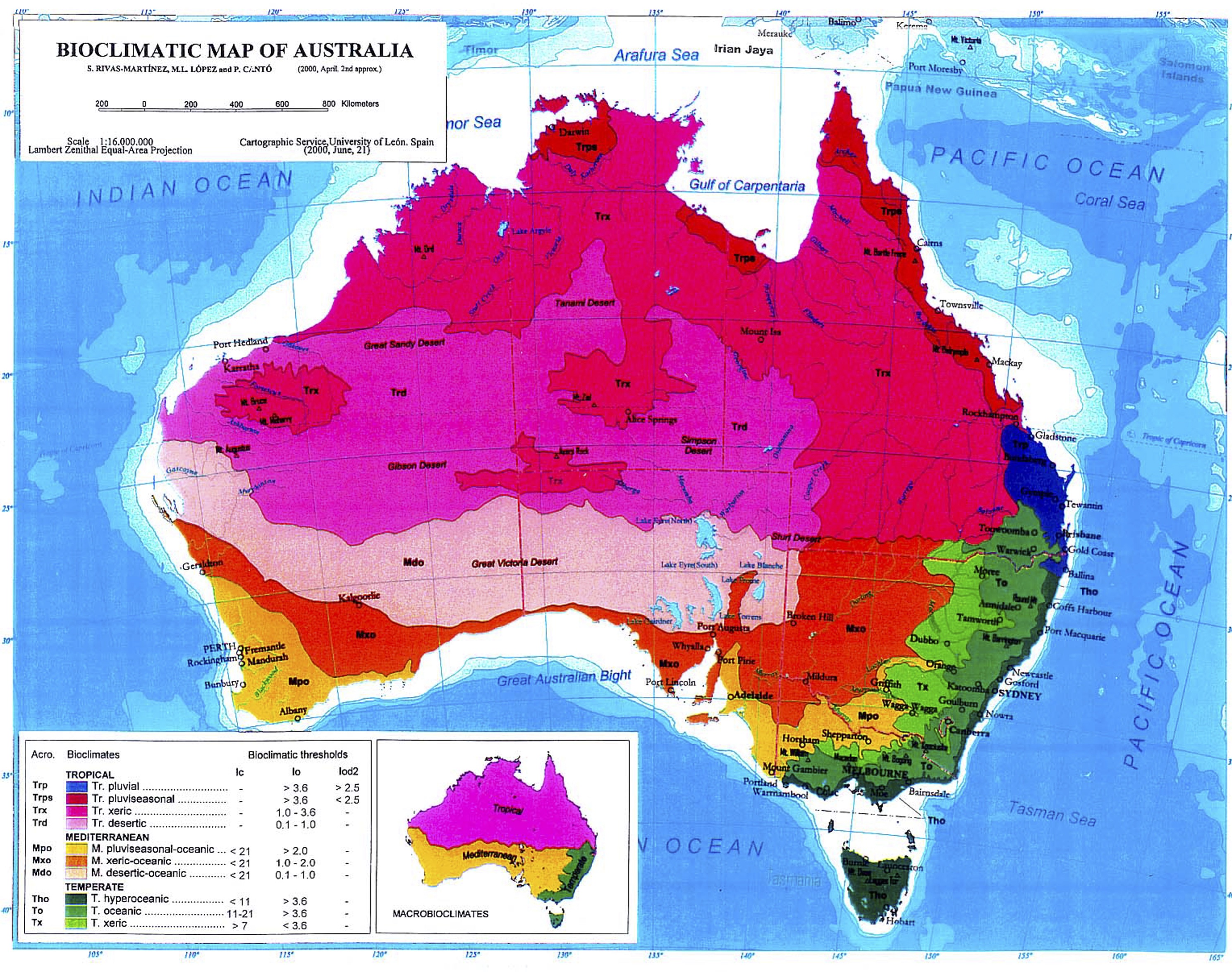
Figure 106. Thermotypes Map of Australia. (Link to its quality file).
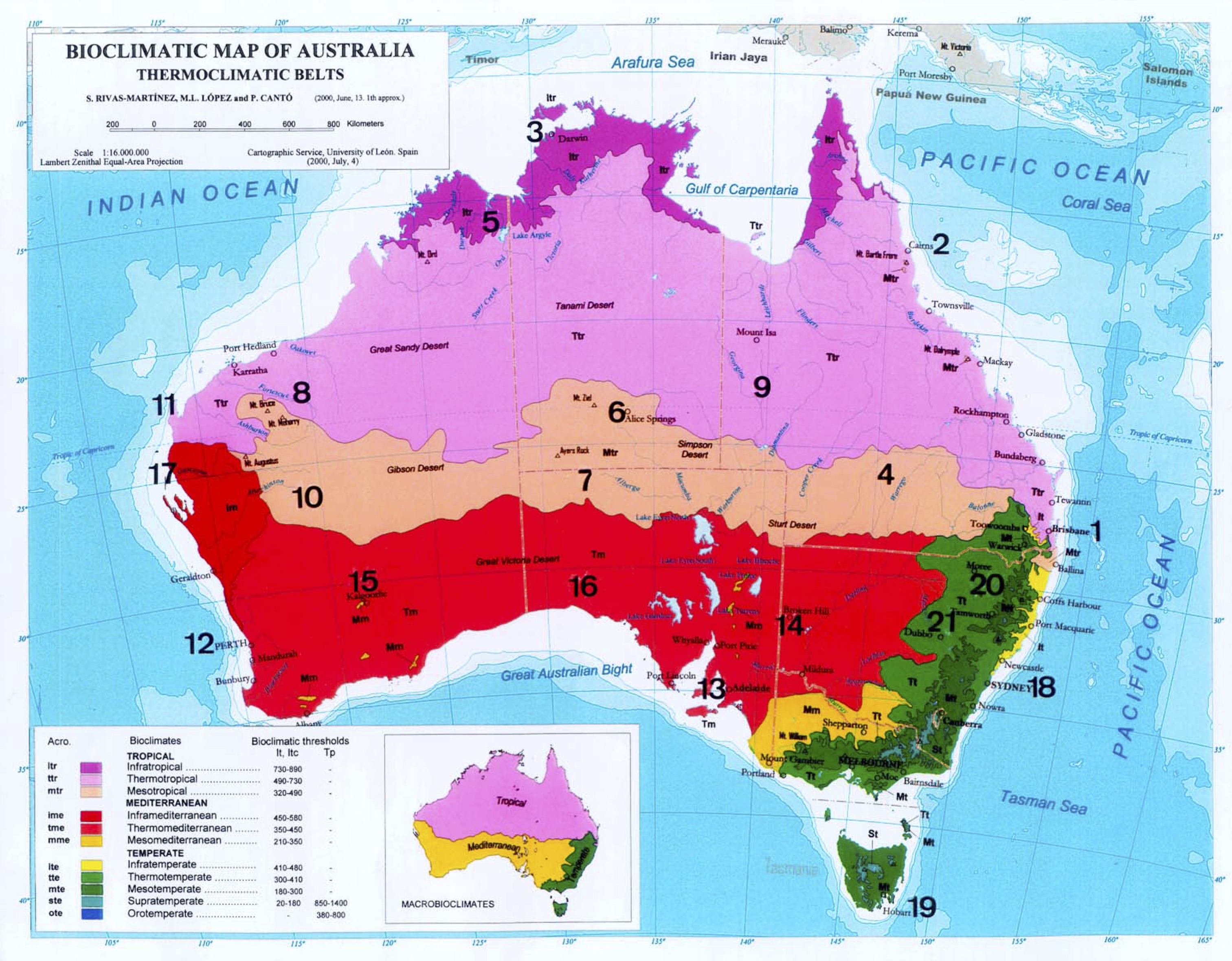

In 2002, Rivas-Martínez, Ogar, Raskovskaja, López
Fernández, Marinish, López, Amezketa and Gelidief presented to Congress
"Itogi i perspektivi rasvitia botanicheskoi nauki v Kazajstane. Alma-Ata, "the Bioclimates Map of Kazakhstan
(Figure 107). Also from Kazakhstan, Rivas-Mart., López, Amezqueta and López
made a Continentality Map (Figure 108), which López Fernández
& López Fernández have just published (Documentos Aljibe "on line", vol.
IV, n7, 16 julio 2017).
Figure 107.- Bioclimatic Map of Kazakhstan. (Link to its quality file).
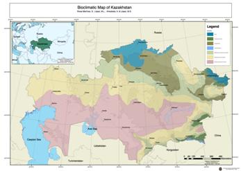
Figure 108. Continentality Map of Kazakhstan.
Most of the country is Eucontinental, while the levels of Semicontinentality
and Subcontinentality only appear in the southeastern mountainous border of the
country. (Link to its quality file).
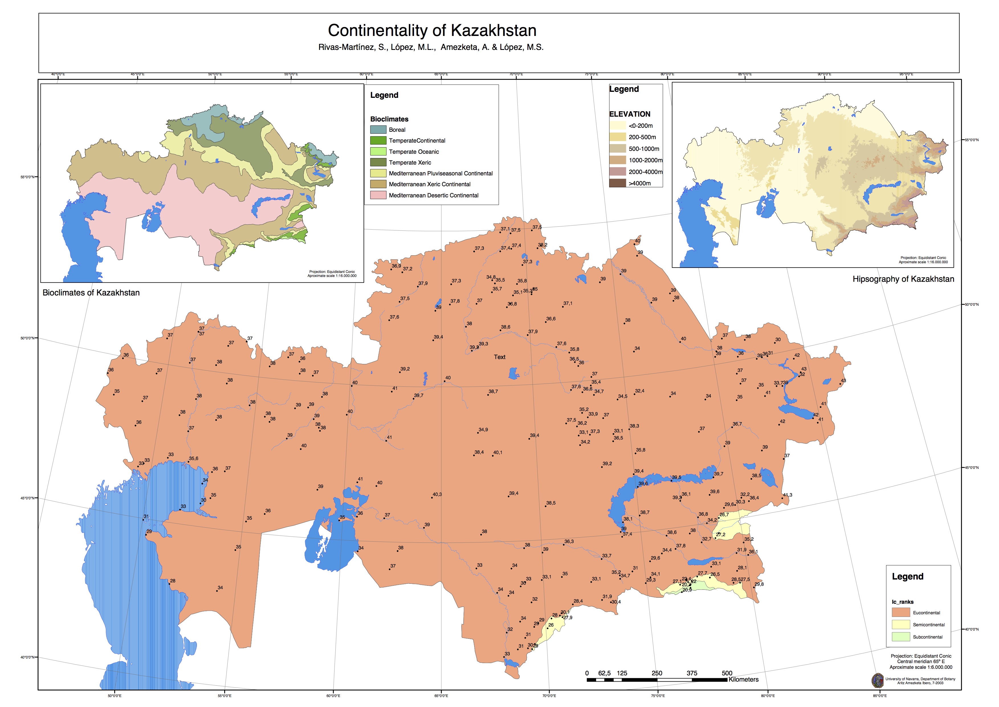
Figure 109.- Far East Russian Macrobioclimates
Map. (Link to its quality file).
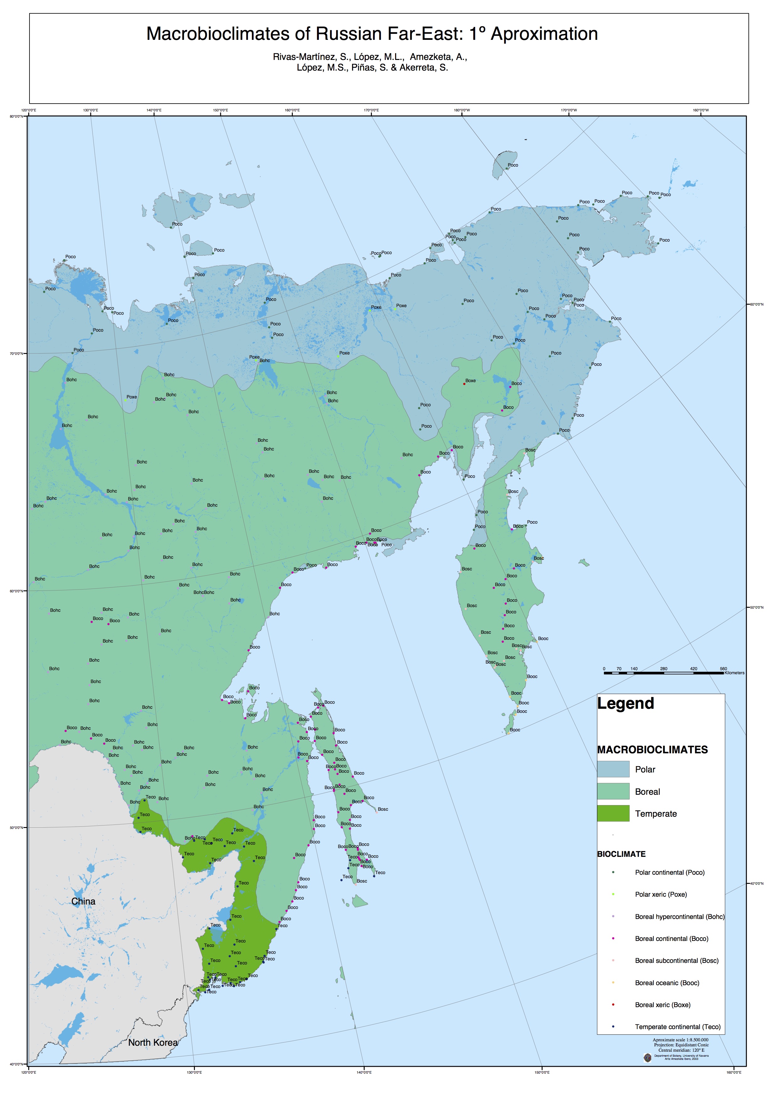
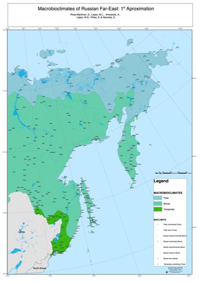
Figure 110. Far East Russian Continentality Map.
(Link to its quality file).
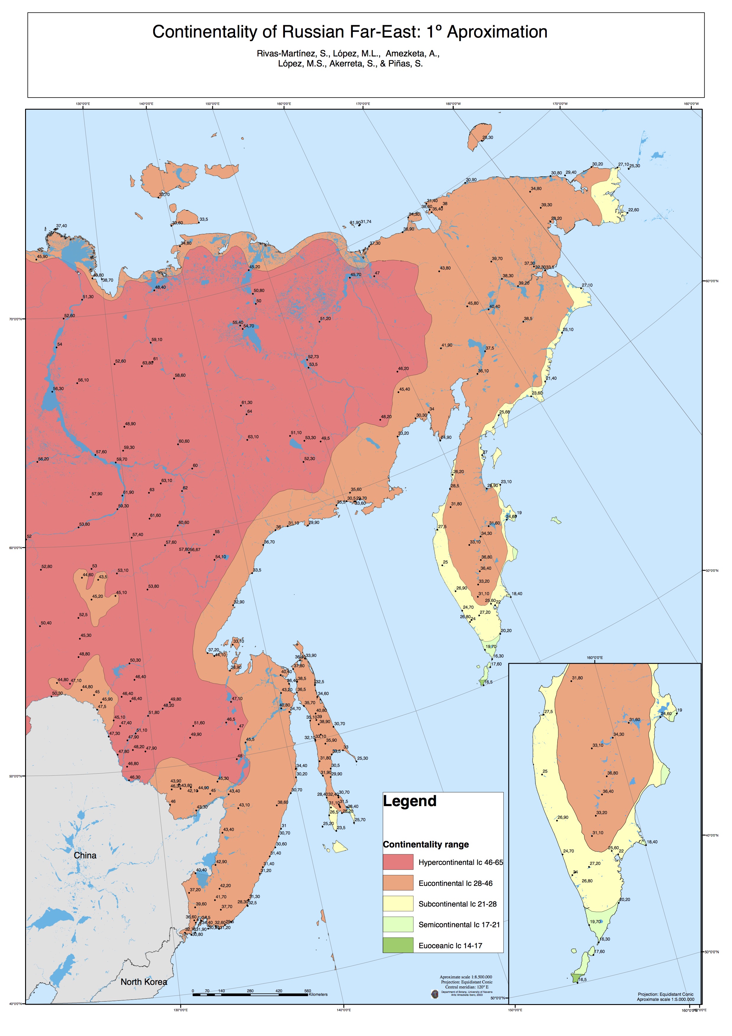
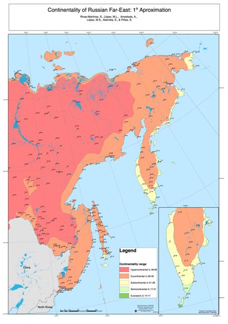
Between 2007 and
2015, a very complete bioclimatic study of Peninsular and Balear Spain, has
been published: we offer it fully in Figures 111-116 - Maps of
Macrobioclimates, of Bioclimates, of Bioclimates / Variants, of Thermotypes, of
Ombrotypes, of Continentality and of Isobioclimates-(Piñas, 2007; López &
al., 2008; Piñas, López et al., 2008 a y b; López, Marco et al., 2015). This
cartographic study is completed with the Continental Map of the same territory,
figure 117, which López Fdez & López Fdez have just published (Documentos Aljibe "on line", vol.
IV, n7, 16 julio 2017).
Figure 111.- Macrobioclimates of Peninsular and Balearic Spain. (Link to its quality file).
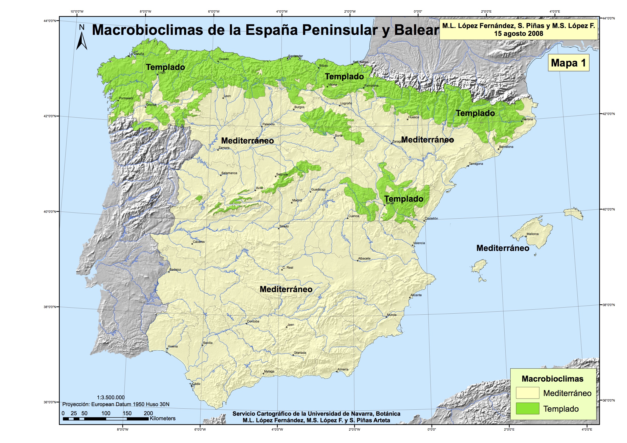
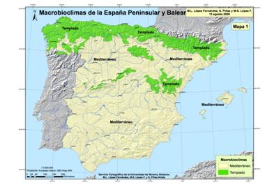
Figure 112.- Bioclimates of Peninsular and Balearic Spain. (Link to its quality file).
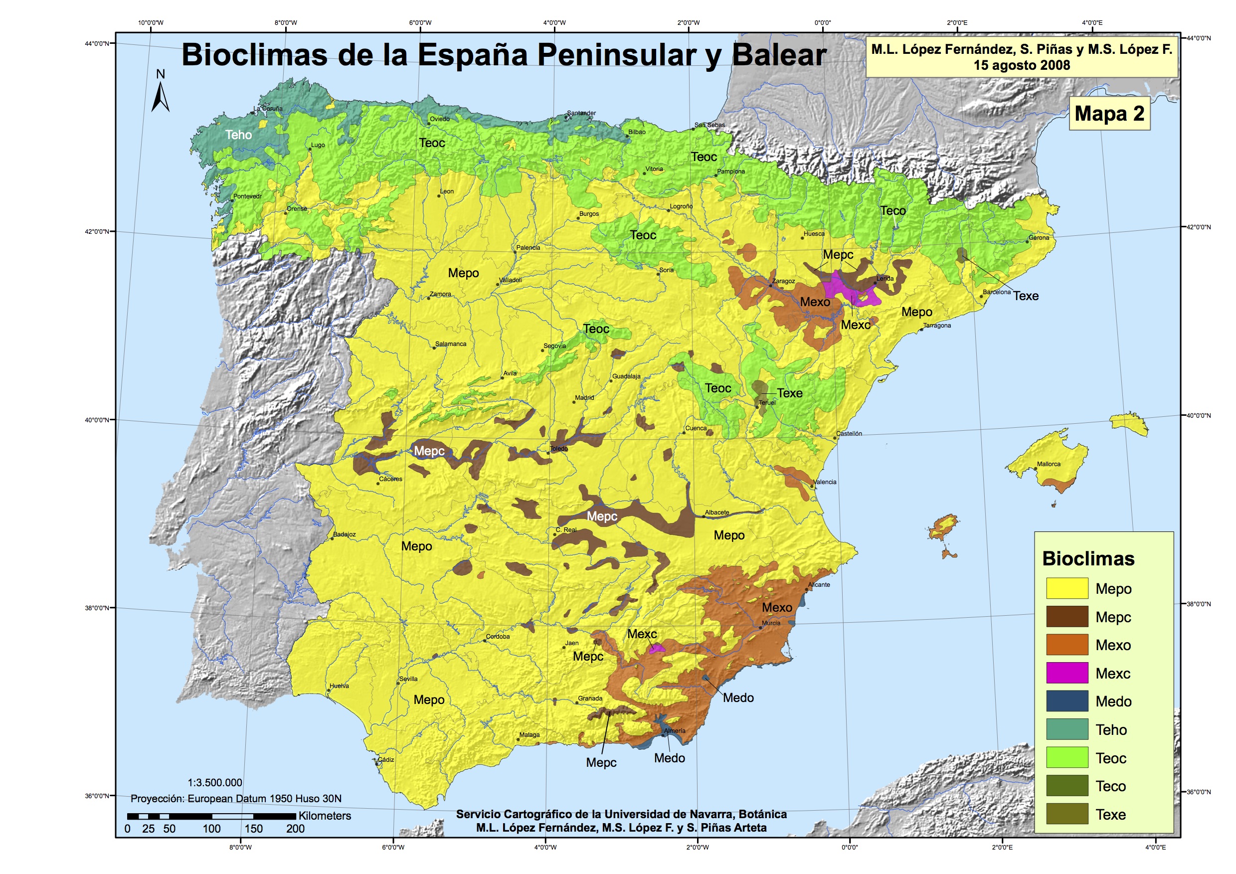
Figure 113.- Bioclimates/Variants Map of Peninsular and Balearic Spain. Note: if the
name of the Bioclimate appears alone, it is understood to mean the Normal
Variant. (Thus: if it is written "Mepo", it means "Mepo
Nor", that is to say, “Bioclimate Mepo Normal Variant”; “Teho” means
“Bioclimate Teho Normal Variant”. (Link
to its quality file).
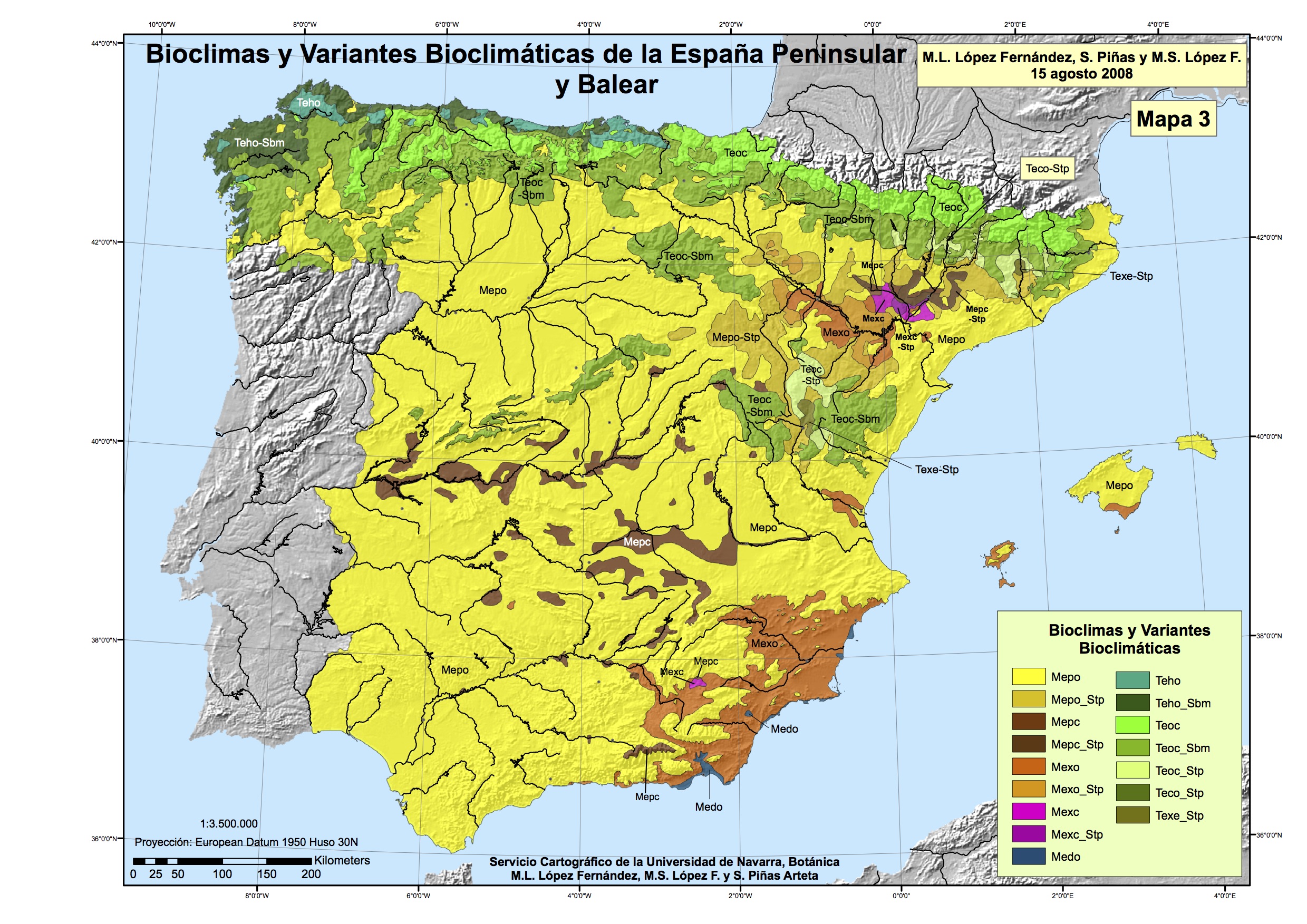
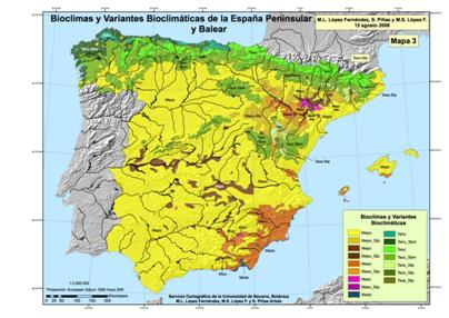
Figure 114.- Thermotypes Map of Peninsular and Balearic Spain. (Link to its quality file).
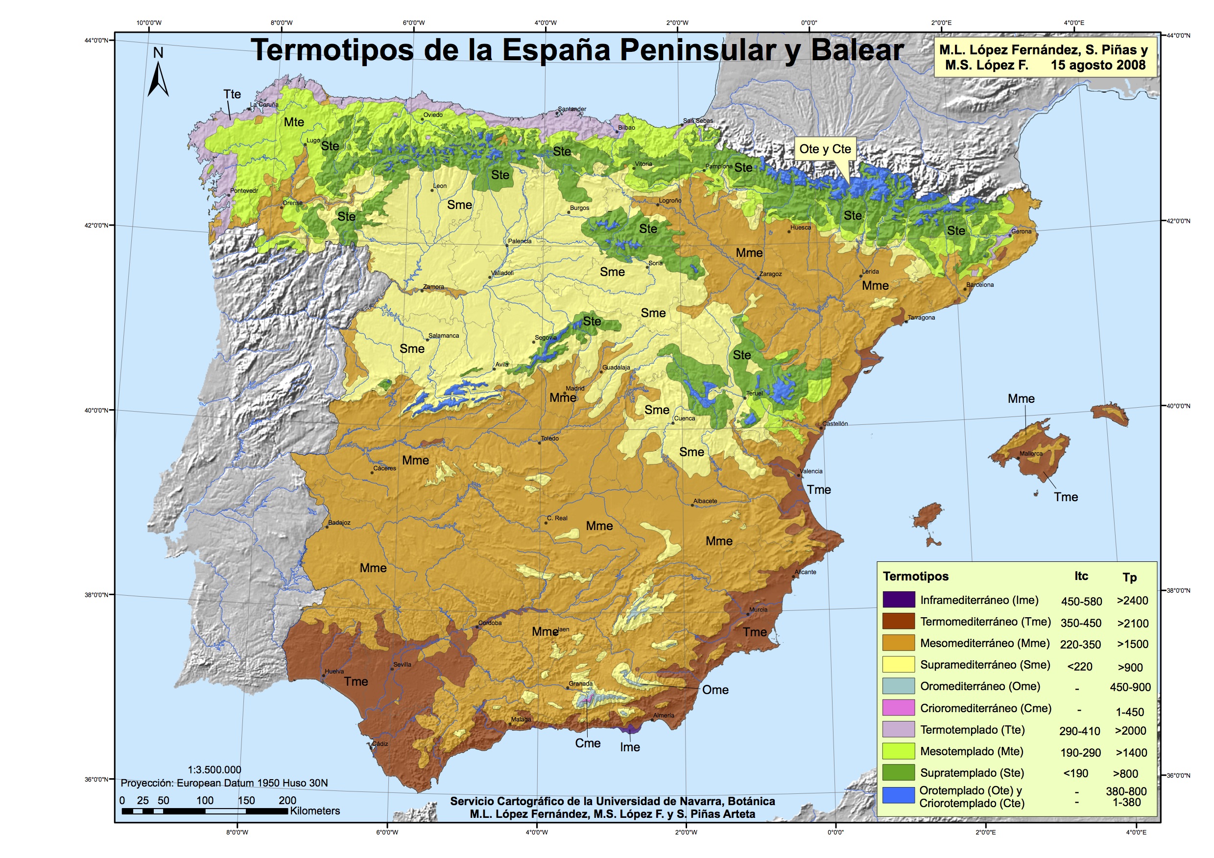
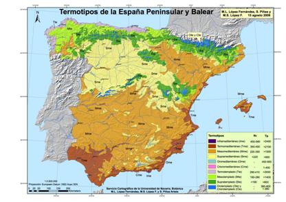
Figure 115.- Ombrotypes Map of Peninsular and Balearic Spain. (Link to its quality file).
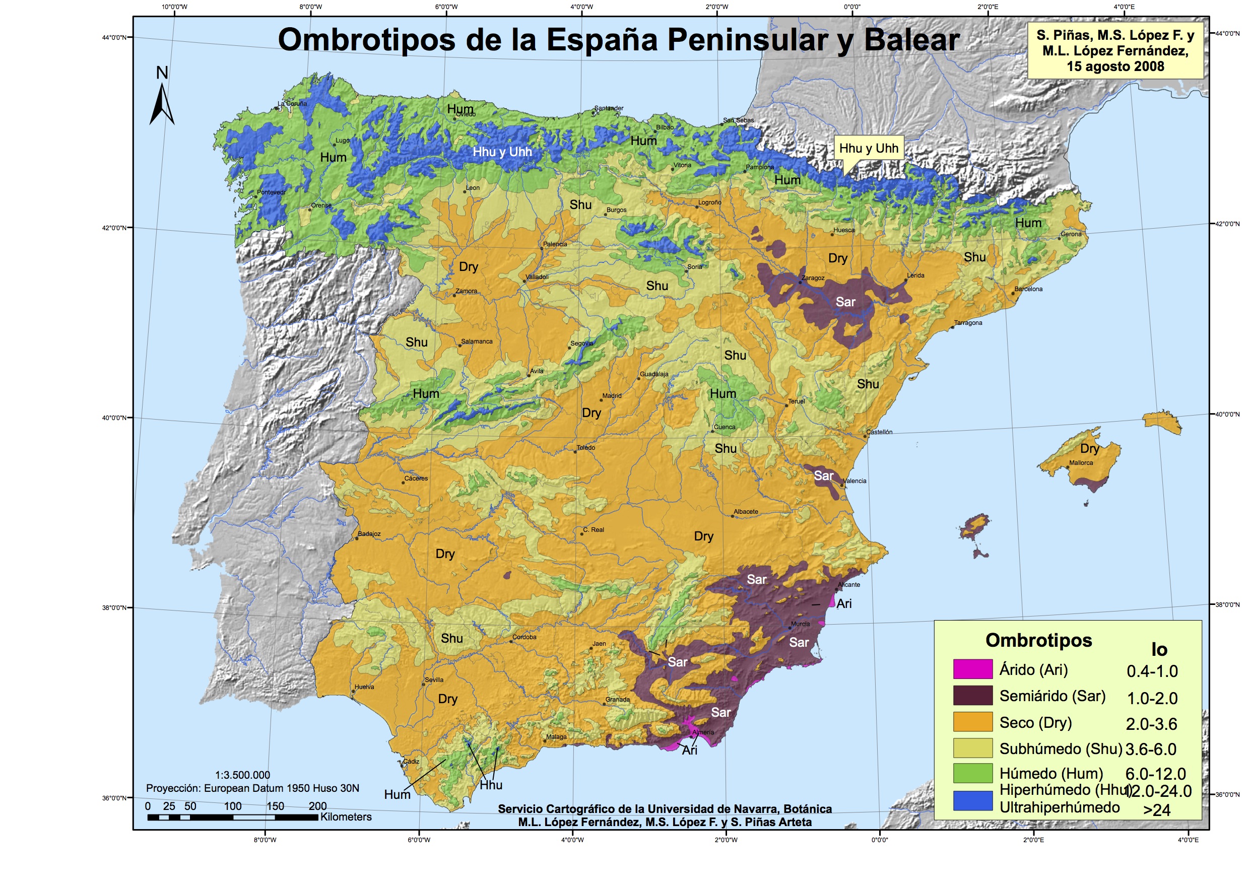
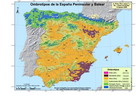
Figure 116.- Isobioclimates Map of Peninsular and Balearic Spain, and its
legend. (Note: in the Isobioclimates without mention of variant Steppic -Stp-,
nor Submediterranean -Sbm-, it is understood that it is the Normal Variant
-Nor-). (Link to its quality
map file and its
quality legend file).
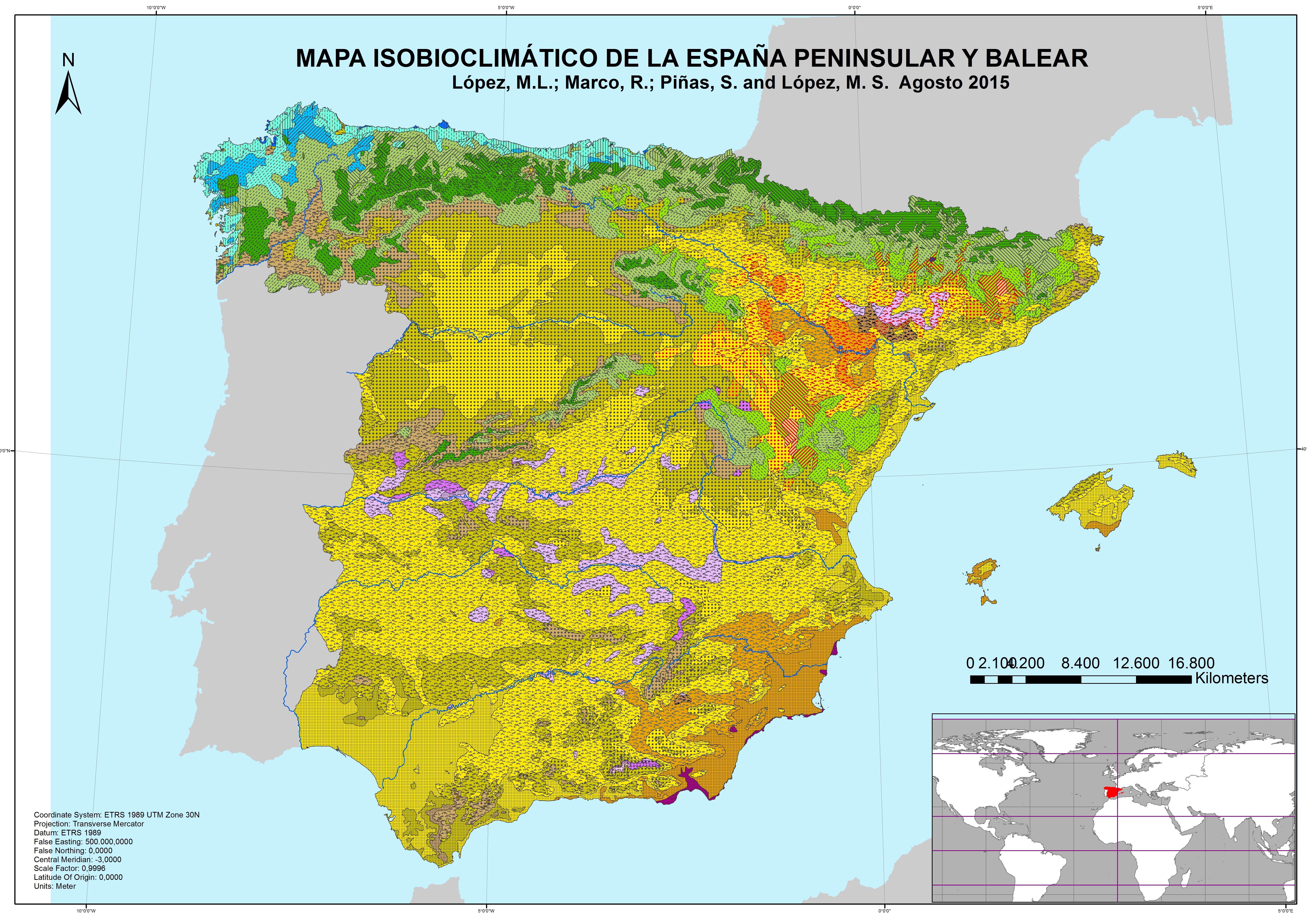
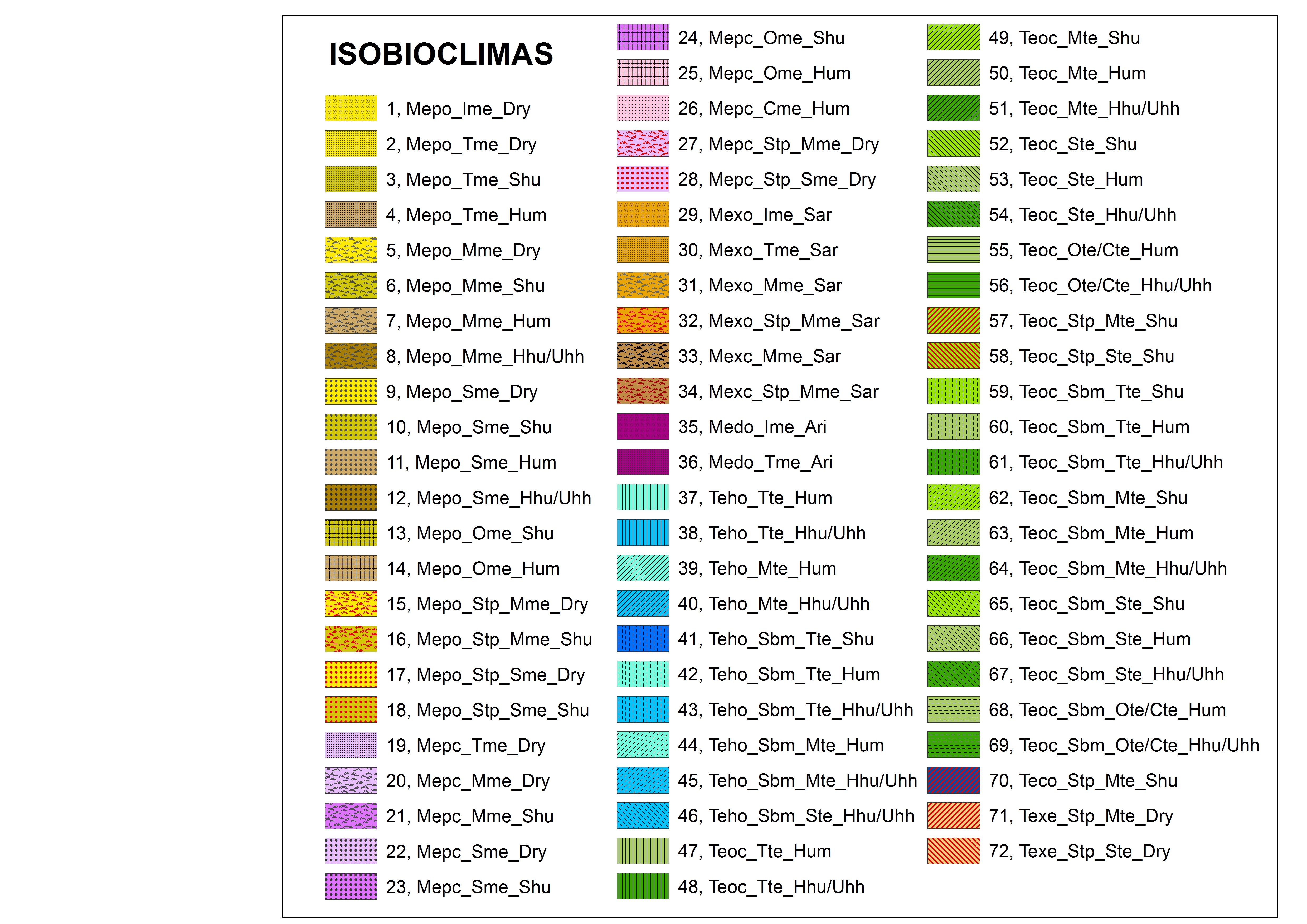
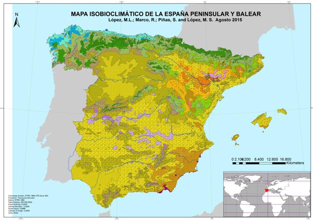
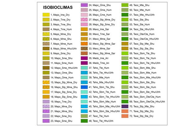
Figure 117.- Continentality Map of Peninsular and Balearic Spain. (Link to its quality file).
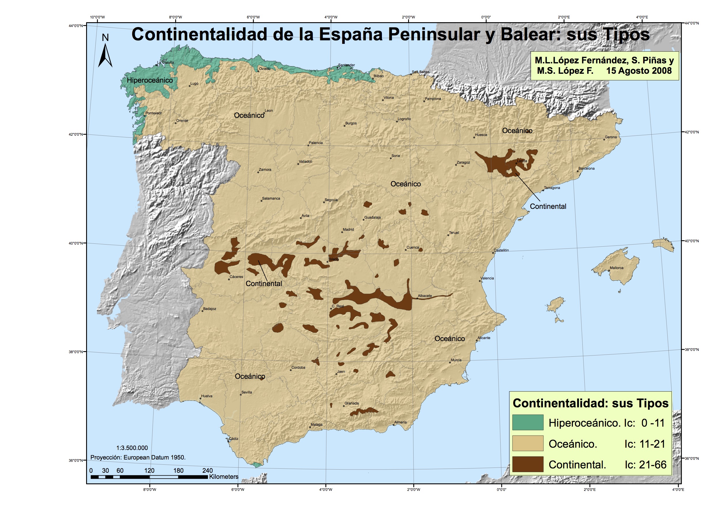
And finally, in
2011, Rivas-Mart. et al. published maps of the worldwide distribution of
Bioclimates, Thermotypes, Ombrotypes and Continentality. It can be very
instructive to see them in the original publication: Rivas-Martínez, S., Rivas
Sáenz, S., Penas, Á. & col. (2011).
13.- PAGINATED GLOSSARY. (Warning: The page numbers refer to the .pdf document,
which can be downloaded from the Web, either at the beginning or at the end of
this work).
|
CONCEPTO |
Page |
|
Angle
of incidence of sun rays |
4 |
|
Annual Positive Precipitation -Pp- |
11 |
|
Annual thermal amplitude |
4, 11, 12 |
|
Antitropical Variant (Ant). |
25, 28, |
|
Biocenosis |
3 |
|
Bioclimates |
24, 25, |
|
Bioclimates / Variants |
17, 24, |
|
Bioclimates
Maps |
141, 142, 145, |
|
Bioclimates/Variants
Map |
146, |
|
Bioclimatic Belts |
17, 31, |
|
Bioclimatic Cartography |
139, |
|
Bioclimatic Horizons |
32, 33, |
|
Bioclimatic Indexes |
6, 11, |
|
Bioclimatic
Synopsis of the Earth |
33, |
|
Bioclimatic Variants |
17, 24, 25, 28, |
|
Bioclimatology |
3 |
|
Bioclimograms |
34, 139 |
|
Bioclimographs |
34, 139 |
|
Bixeric Variant (Bix). |
25, 28, |
|
Boreal Bioclimates |
25, 27, |
|
Boreal Continental Bioclimate |
27, |
|
Boreal Hiperoceanic Bioclimate |
27, |
|
Boreal Hypercontinental
Bioclimate |
27, |
|
Boreal Macrobioclimate |
18, 20, 22, 24, |
|
Boreal Oceánico Bioclimate |
27, |
|
Boreal Subcontinental
Bioclimate |
27, |
|
Boreal Xeric Bioclimate |
27, |
|
Ci: compensation value |
13, 15, 113, |
|
Compensable summer aridity |
102, 105 |
|
Compensated Thermicity, Index
of |
6, 11, 12, 13, |
|
Continental Temperate
Bioclimate |
27, |
|
Continentality / Oceanicity
Index |
6, 11, 12, 14 |
|
Continentality / Oceanicity,
Premise of |
4 |
|
Continentality
Map |
142, 144, 148, |
|
Deserts Premise |
4 |
|
Frost Periods –Pf- |
9, 15, |
|
Frost, Types of |
8 |
|
Global Bioclimatic Diversity |
36, |
|
Hierarchical |
1, 3, 5, 17, 24,
31, |
|
Hypercoceanic Temperate
Bioclimate |
27, |
|
Ic, |
6, 11, 12, |
|
Index of Compensated Thermicity |
6, 11, 12, 13, |
|
Index of Thermicity |
6, 11, 12, |
|
Io |
6, 11, 13, 14, 15 |
|
Iod2 |
14, 15 |
|
Ios |
14, 15, |
|
Ios2 |
14, 15, |
|
Iosc |
14, 15, |
|
Iosc3 |
14, 15, |
|
Iosc4 |
14, 15, |
|
Isobioclimate |
34, |
|
Isobioclimates Map |
147, |
|
It |
6, 11, 12, 15, |
|
Itc |
6, 11, 12, 15, 113, |
|
Latitude |
6, 19, |
|
Latitude,
Premise of Photoperiod/Latitude |
4, |
|
Latitudinal Belts |
6, 7 |
|
Latitudinal Zones |
6, 7 |
|
Macrobioclimates |
17, 18, 20, 24, |
|
Macrobioclimates
Map |
141, 143, 145, |
|
Mediterranean Bioclimates |
25, 26, |
|
Mediterranean Macrobioclimate |
18, 20, 21, 24, |
|
Mediterranean Pluviestacional
Oceanic Bioclimate |
26, |
|
Mediterranean. Desert
Continental Bioclimate |
26, |
|
Mediterranean. Desert Oceanic
Bioclimate |
26, |
|
Mediterranean. Hyperdesertic
Continental Bioclimate |
26, |
|
Mediterranean. Hyperdesertic
Oceanic Bioclimate |
26, |
|
Mediterranean. Pluviestacional
Continental Bioclimate |
26, |
|
Mediterranean. Xeric Continental
Bioclimate |
26, |
|
Mediterranean. Xeric Oceanic
Bioclimate |
26, |
|
Mediterraneity, Premise of |
4 |
|
Normal Variant (Nor). |
25, 31, |
|
Oceanic Temperate Bioclimate |
27, |
|
Ombro-Thermoclimograph |
139 |
|
Ombro-Thermoclimogram |
34, 139 |
|
Ombrothermal Indexes |
6, 11, 13, |
|
Ombrotype |
17, 31, 33 |
|
Ombrotypes Map |
147, |
|
Oroclimates
(Mountain climates), Premise of |
4 |
|
Orogenies, Premise of |
5 |
|
Paginated glossary |
149 |
|
Parameters |
6, 8, 9, 10 |
|
Pav |
15, |
|
Photoperiod / Latitude, Premise
of |
4, |
|
Phytotron |
34, |
|
Plant Activity Period |
6, 8, 9, 15, |
|
Pluvial Hygrophytic, “drought"
level, Variant (Str) |
29, 37 |
|
Pluvial Subhigrophytic, “drought"
level, Variant (Str) |
29, 37 |
|
Pluvial
submesophytic, “drought"
level, Variant (Str) |
29, 37 |
|
Pluviseasonal Mesophytic, “drought"
level, Variant (Str) |
29, 37 |
|
Pluviseasonal Submesophytic, “drought" level, Variant (Str) |
29, 37 |
|
Pluviseasonal Subxerophytic, “drought" level, Variant (Str) |
29, 37 |
|
Pluviseasonal
Xerophytic |
29, 37 |
|
Pluviserotin Variant (Pse). |
25, 28, |
|
Polar Bioclimates |
25, 27, |
|
Polar Continental Bioclimate |
27, |
|
Polar Hyperoceanic Bioclimate |
27, |
|
Polar Macrobioclimate |
18, 20, 23, 24, |
|
Polar Oceanic Bioclimate |
27, |
|
Polar Pergelid Bioclimate |
27, |
|
Polar Semiboreal Variant
(Pose). |
25, 31, |
|
Polar Xeric Bioclimate |
27, |
|
Positive Annual Temperature -Tp- |
10, 16, |
|
Positive Precipitation, Anual -Pp- |
11 |
|
Pp, Annual Positive Precipitation |
11, 15, |
|
Precipitation Parameters |
6, 9, 10, |
|
Premises of the Classification |
3 |
|
Reciprocity, Premise of |
3 |
|
Rhythm of precipitation, annual |
4 |
|
Seasonal Parameters |
6, 9, |
|
Seasonal temperature Variation |
9 |
|
Seasonality of Precipitations |
6, 8, |
|
Seasonality
of Precipitations, Premise of |
4, |
|
Seasonality of Temperatures |
6, 8, |
|
Semitropical Hyperdesertic
Variant (Strhd) |
25, 30, |
|
Steppic Variant (Stp). |
25, 30, |
|
Submediterranean Variant (Sbm). |
25, 30, |
|
Summer aridity |
21, 22, 23, 102,
105 |
|
Temperate Bioclimates |
25, 26, |
|
Temperate Macrobioclimate |
18, 20, 22, 24, |
|
Temperature Parameters |
6, 9, |
|
Thermal and Ombric Variations |
6, |
|
Thermicity, Index of |
6, 11, 12, |
|
Thermotype |
17, 31, 32, |
|
Thermotypes
Map |
141, 146, |
|
Tp, Positive Annual Temperature |
10, 16, |
|
Tropical Bioclimates |
25, |
|
Tropical Desertic Bioclimate |
26, |
|
Tropical Drought Variants
(Str). |
25, 29, |
|
Tropical Hyperdesertic
Bioclimate |
26, |
|
Tropical Macrobioclimate |
18, 20, 21, 24, |
|
Tropical Pluvial Bioclimate |
26, |
|
Tropical Pluviseasonal
Bioclimate |
26, |
|
Tropical Xeric Bioclimate |
26, |
|
Types of Frost |
8 |
|
Types of frost. |
6, 8, |
|
Variants, Bioclimatic |
17, 24, 25, 28, |
|
Xeric Temperate Bioclimate |
27, |
14.- TABLE
OF CONTENTS
1.-
INTRODUCTION
2.- PREMISES OF THE BIOCLIMATIC CLASSIFICATION OF THE
EARTH, RIVAS-MARTÍNEZ & al. (2011)
2.1.-
Reciprocity
2.2.-
Photoperiod / Latitude
2.3.- Continentality / Oceanicity - Annual thermal amplitude
2.4.- Seasonality of Precipitation
2.5.- Mediterraneity
2.6.- Deserts
2.7.- Oroclimates (Mountain climates)
2.8.- Orogenies
3.-
BASIC COMPONENTS FOR THE WORLDWIDE BIOCLIMATIC CLASSIFICATION
3.1.- Latitude:
Latitudinal Zones and Waists
3.2.-
Seasonality of temperatures and rainfall. Period of plant activity. Types of
frost.
3.3.-
Parameters:
3.3.1.- Seasonal Parameters
3.3.2.- Temperature Parameters
3.3.3.-
Precipitation Parameters
3.4.- Bioclimatic
Indexes
3.4.1.- Continentality / Oceanicity Index: Annual
thermal amplitude -lc-
3.4.2.- Index of Thermicity -It- and Index of
Thermicity Compensated -Itc-
3.4.3.-
Ombrothermic Indexes -Io-
3.5.-
Alphabetical list of the abbreviations that designate the Parameters and the
Bioclimatic Indexes,
4.- WORLDWIDE BIOCLIMATIC CLASSIFICATION
4.1.- First hierarchical level of the Classificacion:
Macrobioclimates
4.1.1.-
Tropical Macrobioclimate
4.1.2.-
Mediterranean Macrobioclimate
4.1.3.-
Temperate Macrobioclimate
4.1.4.-
Boreal Macrobioclimate
4.1.5.-
Polar Macrobioclimate
4.1.6.- Macrobioclimates
Continental Distribution
4.2.- Second hierarchical level of the
Classification: Bioclimates /
Variants
4.2.1. Bioclimates
4.2.1.a) Tropical Bioclimates
4.2.1.b) Mediterranean Bioclimates
4.2.1.c)
Temperate Bioclimates
4.2.1.d) Boreal
Bioclimates
4.2.1.e)
Polar Bioclimates
4.2.2.-
Bioclimatic Variants
4.2.2.a) Pluviserotin
Variant (Pse)
4.2.2.b)
Antitropical Variant (Ant)
4.2.2.c) Bixeric
Variant (Bix)
4.2.2.d)
Tropical Drought Variants (Str)
4.2.2.e) Semitropical Hyperdesertic Variant
(Strhd)
4.2.2.f) Steppic
Variant (Stp)
4.2.2.g) Submediterranean
Variant (Sbm)
4.2.2.h) Polar
Semiboreal Variant (Pose)
4.2.2.
I) Normal Variant (Nor)
4.3.- Third
hierarchical level of the Classification: Bioclimatic Belts -Thermotypes and
Ombrotypes-
4.3.1.- Thermotypes
4.3.2.- Ombrotypes
5.-
BIOCLIMATIC SYNOPSIS OF THE EARTH
6.-
ISOBIOCLIMATE
7.-
BIOCLIMOGRAMS
8.-
APPROACH to the GLOBAL BIOCLIMATIC DIVERSITY
8.1.- Diversity at Macrobioclimate level 36
8.2.-
Diversity at Bioclimate/Variant level 36
8.3.-
Diversity at Bioclimatic-Belt level 36
8.4.- Examples of Global
Bioclimatic Diversity at the Macrobioclimate / Bioclimate / Bioclimatic Varian
levels 39
9.- ASSESSMENT
OF SUMMER ARIDITY, WITH EXAMPLES
9.1.- Assessment of summer aridity
9.2.- Examples for the valuation of summer aridity
10.- Itc
and Ci CALCULATIONS
11.- PRACTICAL EXAMPLE of a
meteorological station complete bioclimatic characterization, with the -use of
the Synoptic Table.
11.1.- Climatic data of departure
11.2.- Bioclimatic diagnosis
of a weather station
11.2.a.- Location of the weather station: Latitude,
longitude and altitude
11.2.b.- Calculation of the
necessary values and indexes
11.2.c.- Recognition of the bioclimatic units of the
station, using the General Synoptic Table
11.2.d.- Expression of the
complete bioclimatic diagnosis -Isobioclimate-.
11.3.- Synthesis and graphic
expression of bioclimatic study: Bioclimograph
12.- CARTOGRAFÍA BIOCLIMÁTICA
13.- PAGINATED
GLOSSARY
14.- TABLE
OF CONTENTS
15.-
BIBLIOGRAPHY
15.- BIBLIOGRAPHY
Gaussen, H. et F. Bagnouls (1952). L’indice
xérothermique. Bull. de l’Assoc. de géographes français. 1952, pp. 10-16.
López Fernández, ML & López Fernández, MS. (2008)
Ideas básicas de “Global Bioclimatics”, del Prof. Rivas-Martínez: Guía para
reconocer y clasificar las unidades bioclimáticas. Publ. Biol. Univ. Navarra,
Ser. Bot., 17:3-188.
López
Fernández, M.L.& López Fernández, M.S. (2017). “Manual y
Guía de Bioclimatología Mundial”. Documentos Aljibe “on-line”, vol.
IV, n.6, 13 de abril de 2017. Ciudad Real. Edita Sociedad Surcos. Depósito
Legal: CR 820-1986- - ISBN 84-398-6347-0 ISSN
2445-1304. http://www.naturalezenhispania.com.
López
Fernández, M.L., López F., M.S., Piñas, S. (2009). “A Bioclimatic & Cartographic Formulation of
Climate for Biogeography”. Poster Presentation, 4rd. Biennal
Conferen. of IBS. Mérida, México
López
Fernández, M.L., Marco, R., Piñas, S., López, S. (2015). “Mapa Isobioclimático
de la España Peninsular y Balear”. Documentos Aljibe “on line”, vol. II, nº 4.
Ciudad Real, España. Edita Sociedad Surcos. Depósito Legal: CR 820-1986- - ISBN 84-398-6347-0
ISSN 2445-1304. http://www.naturalezenhispania.com.
López
Fernández, M.L., Piñas, S., López F., M.S. (2008). “Macrobioclimas, Bioclimas y
Variantes Bioclimáticas de España Peninsular y Balear”. Publicaciones de
Biología, Universidad de Navarra, Serie Botánica, 17, 229-236.
López
Fernández, M.S. & López Fernández, M.L. (2017). “Bioclimatología: Estudio
comparado de Continentalidad en España Peninsular, Kazakjistán y Lejano Oriente
de Rusia”. Documentos Aljibe “on-line”, vol. IV,
n.7, 16 julio 2017. Ciudad Real. Edita Sociedad Surcos. Depósito
Legal: CR 820-1986- ISBN 84-398-6347-0 ISSN 2445-1304. http://www.naturalezenhispania.com
Piñas,
S. (2007). Bioclimatología de la
España Peninsular y Balear, y su
Cartografía. Tesis Doctoral. 110 pp. y anexos. Universidad de Navarra. Manuscrito
inédito.
Piñas,
S., López F., M.S., López Fernández, M.L. (2008a). “Termotipos de la España
Peninsular y Balear, y su cartografía”. Publicaciones de Biología, Universidad
de Navarra, Serie Botánica, 17, 237-242.
Piñas,
S., López F., M.S., López Fernández, M.L. (2008b). “Ombrotipos de la España
Peninsular y Balear, y su cartografía”. Publicaciones de Biología, Universidad
de Navarra, Serie Botánica, 17, 243-248
Rivas-Martínez,
S. (1987). Nociones sobre Fitosociología, Biogeografía y Bioclimatología. In:
Peinado, M & S. Rivas-Martínez (eds.) La vegetación de España: 19-45. Ed.
Rivas-Martínez,
S. (2004). Global Bioclimatics (Clasificación Bioclimática de la Tierra)
(Versión 27-08-2004). www.globalbioclimatics.org.
Rivas-Martínez,
S. (2008). Global Bioclimatics (Clasificación Bioclimática de la Tierra). www.globalbioclimatics.org.
Rivas-Martínez,
S., López, M.L. & Cantó, P. (2000a). Bioclimatic Map of Australia: Macrobioclimate and
Bioclimate. Cartographic Service, University of León, Spain.
Rivas-Martínez, S., López, M.L. & Cantó, P.
(2000b). Bioclimatic Map of Australia. Thermoclimatic Belts. Cartographic
Service, University of León, Spain
Rivas-Martínez, S., López Fernández, M.L., Amezketa,
A., López, M.S., Aquerreta, S., Piñas, S. (2003). “Macrobioclimates,
Bioclimates, Thermotypes, Ombrotypes and Continentality Maps of Far East
Russia”. En Phytogeography of Northeast Asia: task for the 21st century.
Vladivostok (Rusia).
Rivas-Martínez, S., Ogar, N., Raskovskaja, E., López
Fernández, M.L., Marinish, O., López, M., Amézketa Ibero, A., & Gelidief,
B. (2002). Bioclimaticheskaja
Karta Kazakhstaja. (Mapa Bioclimático de Kazakhstán). En Itogi i perspektivi
rasvitia botanicheskoi nauki v Kazajstane (Materiali mezdunarodoi nauchnoi
konferencii, pocviachshenou 70-letiiu Instituta Botaniki i Fitointrodukcii), Alma-Ata
(Kazakhstán), 259-261.
Rivas-Martínez,
S. & Rivas-Saenz, S. (1996-2017). Worldwide Bioclimatic Classificacion System. Phytosociological Research
Center, Spain. http://globalbioclimatics.org/
Rivas-Martínez,
S., Rivas Sáenz, S., Penas, Á. & col. (2011). Worldwide Bioclimatic Classification System.
Global Geobotany, 1: 1-634 + 4 Maps
Walter, H.
& Lieth, H. (1967). Klimadiagramm-Weltatlas. Gustav
Fischer Verlag, Jena 1967.
© López Fernández, María Luisa &
López Fernández, María Soledad.
.
___________________________________________________________________________________________________________
Edita: Sociedad SURCOS,
Avda. Torreón, nº 1 13001 Ciudad Real - Depósito Legal: CR 820-1986- - ISBN
84-398-6347-0 ISSN en tramitación- Aviso
Legal